Metaphysics
Table of Contents
Metaphysics (2022)
(dice and dominoes)
Showcase
Music: The Moldau (Bedřich Smetana)
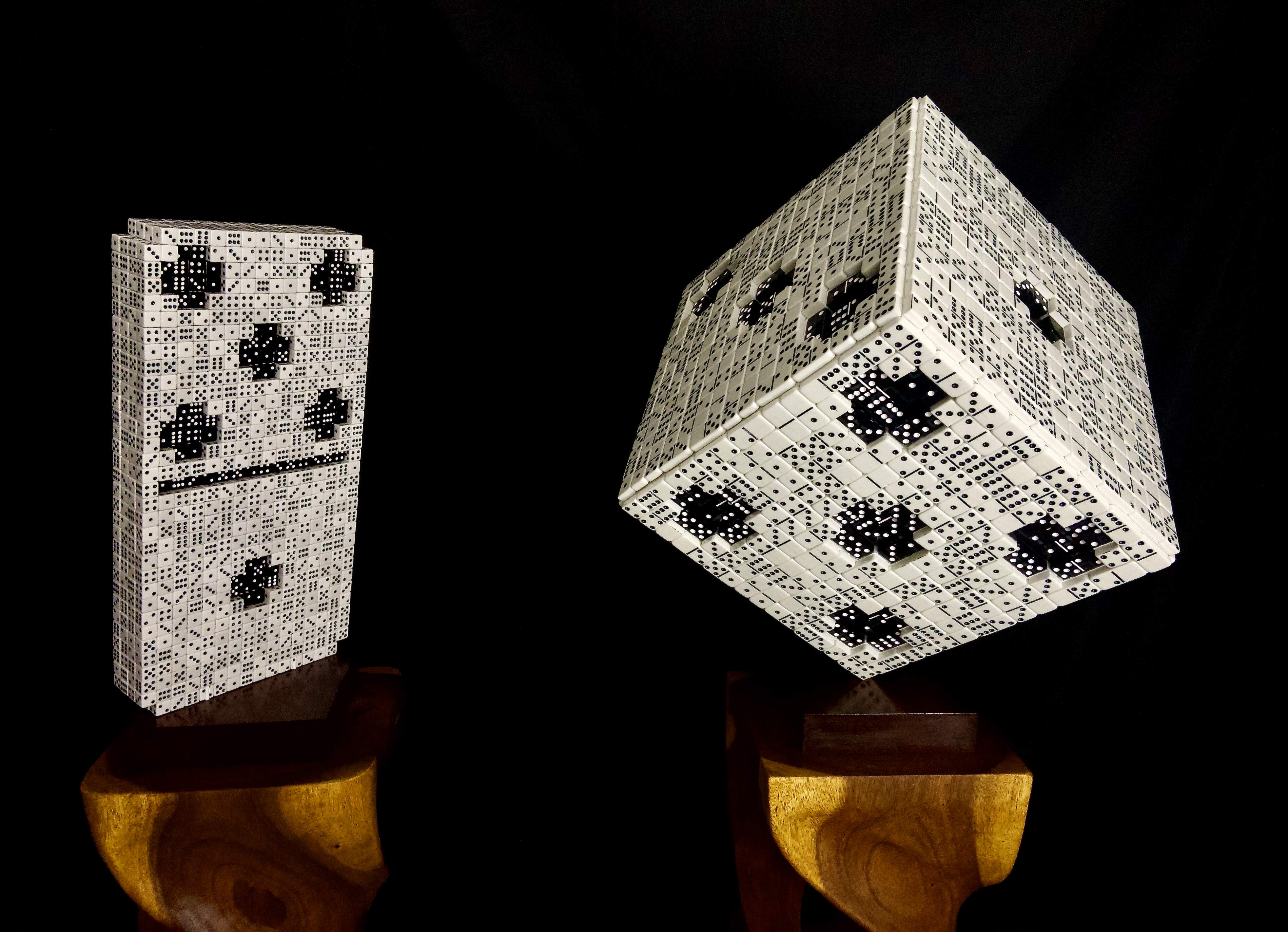
Metaphysics is a pair of sculptures: a domino made of dice, and a die made of dominoes.
This page explains the Meaning, Making, Math, and Code of Metaphysics. It's a very long page, so use the table of contents to more easily navigate.
A secret pattern that only reveals itself in the dark!
Jump to Dimensionality and Topology for details
I plan to someday build a much larger version of Metaphysics. The sculptures you see here are works in their own right, but I consider them small models — in fact, the smallest possible models I could have built.
In creating these models, I completed much of the research and developed much of the technical infrastructure I'll need to make the larger versions. For example, I can use the exact same math and code at larger scales by simply changing a few parameters.
My dream is to install the larger sculptures in a very specific location at Stanford (my alma mater): Lomita Mall Green North, a small grassy area between the Physics department and the Math and Philosophy departments:
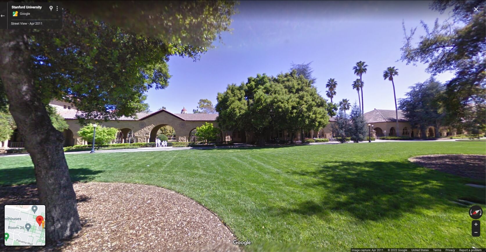
Stanford University: Lomita Mall Green North
(Google Street View)
I can think of no more fitting home for Metaphysics.
A major goal of my work so far is inspiring enthusiasm and support for this project. If you want to support my efforts, and especially if you could help put me in touch with the right people at Stanford, please reach out to me.
Thank you!
Meaning
Metaphysics is a yin and yang of sorts that explores the duality between determinism and randomness, between fate and chance. It manifests the interplay between fundamental, microscopic laws and emergent, macroscopic properties. Its title references both metaphysics the philosophical discipline and a meta perspective on physics.
Domino of Dice
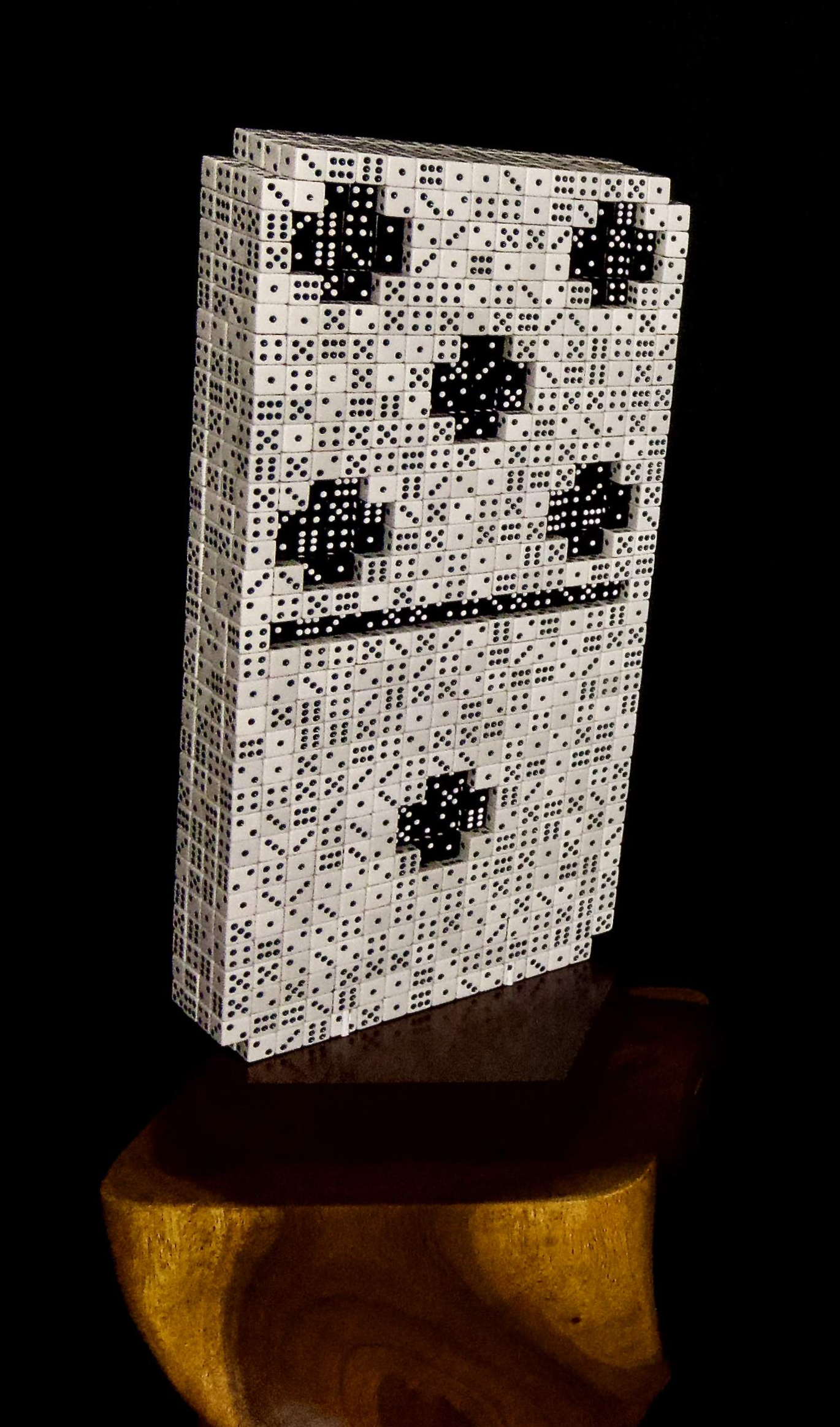
Domino of Dice
The domino of dice is at first glance a contradiction. A domino is the quintessential symbol of determinism, of certainty, of fate. Dominoes fall; they don't un-fall. Playing dominoes amounts to lining them up end to end, numbers matching. A die is almost opposite: it's the quintessential symbol of randomness, of probability, of chance. Dice roll unpredictably. Playing dice amounts to betting on entirely stochastic outcomes. And yet here we see a domino composed of dice! What sense could this possibly make?
Quantum Mechanics, Entropy, and Emergence
As strange as it may seem, the domino of dice reflects our best understanding of modern physics, of how the universe works. Quantum mechanics, in particular, tells us that at the scale of the tiny components of our world — electrons, atoms, and fields — there is probability, not definiteness. In fact, this randomness is irreducible, as the famous Heisenberg uncertainty principle makes concrete.
The Heisenberg uncertainty principle states:
To understand why this means uncertainty is irreducible, it's not necessary to know what these quantities mean. It's enough to see that the left side of the equation corresponds to uncertainty, and the on the right side is greater than zero. So, this equation says uncertainty has a nonzero lower bound.
But for those who are curious to know the details, and are the standard deviations of position and momentum, respectively — e.g. of a particle). And is the reduced Planck constant. Position and momentum are complementary variables, meaning it's impossible to measure them both with perfect accuracy at the same time.
The uncertainty in what we observe in experiments is not due to a lack of skill. No matter how good we ever become at making measurements, that randomness will never vanish. Achieving 100% certainty is impossible not just in practice but in principle.
But quantum mechanics is just a theory, so might it be wrong? Yes, but only in a very limited sense.
Over a century after quantum mechanics was formulated, not a single experiment has contradicted it. This means any future theory that suceeds quantum mechanics must also agree with all of those experiments. In other words, it must expand on quantum mechanics rather than invalidate it, in the same way that Einstein's theory of gravity (general relativity) expanded on Newton's theory of gravity but didn't invalidate it. (Newton's theory is so accurate that it's still used to send rockets into space!)
And yet, at the scale of human beings, the world exhibits none of this randomness, despite being made of smaller pieces that do. The macroscopic universe has a predictablity that the microscopic universe lacks. Eggs crack; they don't un-crack. Wood burns; it doesn't un-burn. Dominoes fall; they don't un-fall.
How can this be, that small pieces with randomness constitute a large object without it? The reasons are complex, but there are two worth remembering:
- Roughly speaking, uncertainty is lower when mass is higher, and everything in our everyday experience is large compared to the tiny particles of nature, just as the domino is large compared to the dice that make it up.
- Entropy tends to increase, and the universe started in a low entropy state. Entropy simply refers to the number of possibilities. There are far more ways for eggs to be cracked than whole, for wood to be burnt than not, for dominoes to be fallen than upright. So, even when what happens is random, it tends toward higher entropy states.
The Unmoved Mover
There's also a philosophical dimension to the domino of dice. It's perched precariously on its balance point, in unstable equilibrium, with its center of mass directly over the axis of rotation. The slightest breeze would make it fall, but in which direction we can only guess. But usually, when we think of dominoes falling, we imagine a long line of them, one hitting the next, hitting the next, and on and on. But here, there's only one domino, which begs the question: if it falls, what caused it to?
Dominoes falling down
This manifests the age old philosophical concept of the "unmoved mover", introduced by Aristotle — in a work fittingly called Metaphysics. The unmoved mover is an attempt at answering the fundamental dilemma of determinism. If everything is ultimately a chain of causes and effects, what was the first cause? What happened without anything happening prior? That quandary, still unresolved well over two milennia since Aristotle made his best effort, is what this sculpture contemplates with its delicate balancing act.
Die of Dominoes
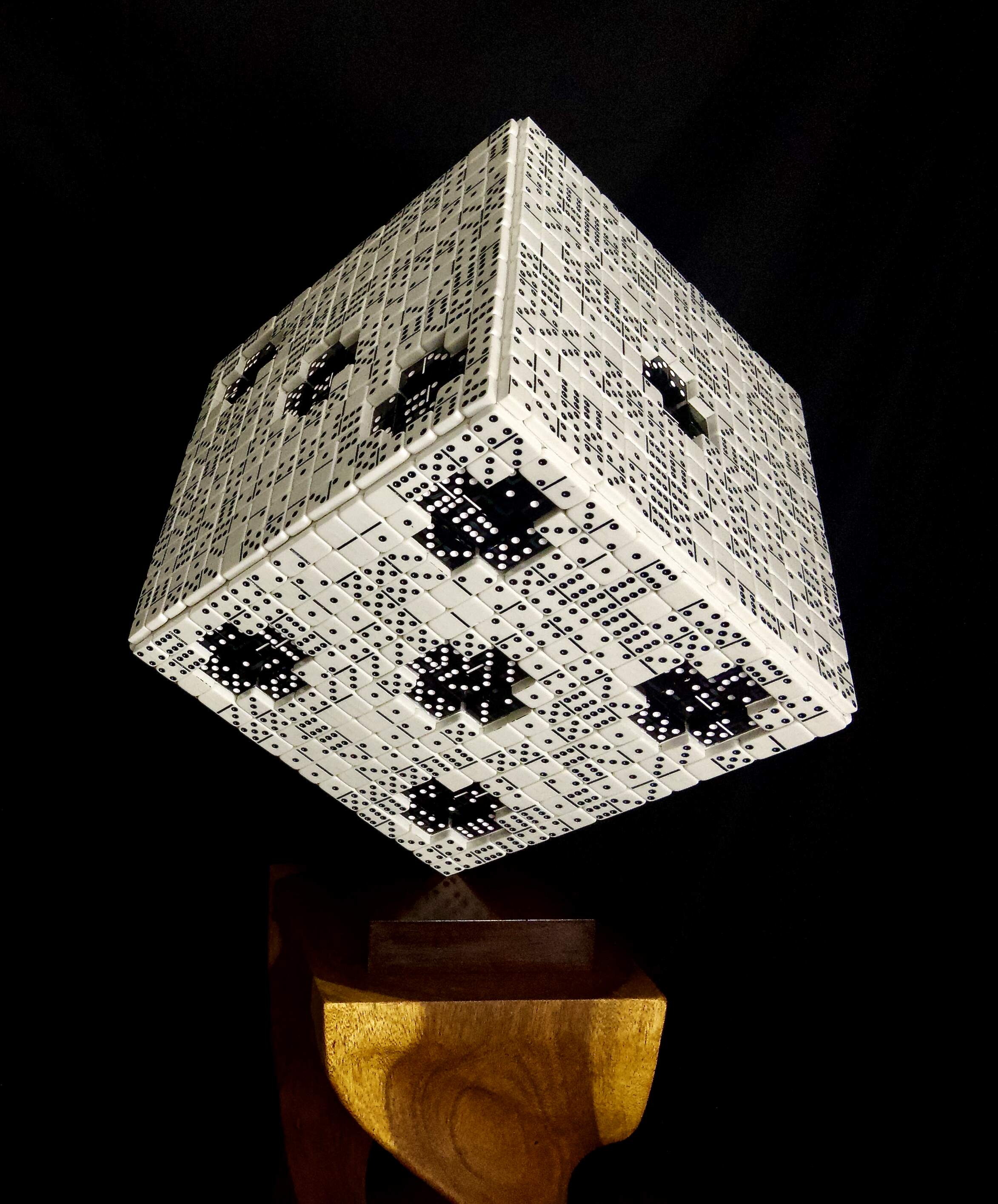
Die of Dominoes
The die of dominoes is also at first glance a contradiction, but one of a different sort. Its constituent pieces are entirely predictable: dominoes lined up end to end with matching numbers. And yet its whole is entirely probabilistic: a die, in mid roll, that could land on any side. Since the domino of dice reflects our best understanding of how the universe works, does the die of dominoes represent the opposite?
Chaos, Information, and Emergence
On the contrary, it also represents our best understanding of modern physics. Chaos theory shows us that, even if the fundamental laws of nature were entirely deterministic, it would still be impossible to predict what would happen in general. Events at larger scales are highly probabilistic, if not completely random. Such randomness emerges from small scale components, even if those components are entirely predictable.
More specifically, chaos says that any difference between the state of a system and what we measure it to be will quickly become extremely large as the system evolves. In a chaotic system, an arbitrarily small difference magnifies exponentially quickly, so that in short order the behavior of the system becomes totally unpredictable.
A simple example of a chaotic system is the double pendulum (or 2-pendulum): a pendulum attached to a pendulum. The animation below shows ten 2-pendula, each beginning at a position meters away from its nearest neighbor. Even with a perturbation this absurdly small — a tenth of a picometer! — the 2-pendula quickly diverge from each other on the order of meter, easily visible to the naked eye.
Ten 2-pendula
Perturbed by increments of 0.1 picometers
In general, -pendula are chaotic when , and they diverge seemingly ever more quickly. As one example, the animation below shows five 5-pendula, each peturbed by the same distance as above ( meters). As with the 2-pendula, the 5-pendula diverge rapidly (and are entertaining to watch!).
Five 5-pendula
Perturbed by increments of 0.1 picometers
Akin to the uncertainty of quantum mechanics, this unpredictability is unavoidable and irreducible. It's not for lack of computing power or calculational ability or cleverness. It's simply the way the world is. No matter how good we ever become at making measurements, we will be unable to make accurate predictions at large scales and over long time horizons. Chaos will still reign.
There's another, more familiar sense in which uncertainty emerges from certainty, and it's due to lack of information. A rolling die in the real world, where friction and dampening effects will ultimately cause the die to stop rolling, is not a chaotic system. In principle, we could predict which number it would settle on, if we knew with great accuracy how fast and in which direction it was spinning, how far it was above the surface, the material properties of the surface, and so on. But in practice, of course, we typically have no access to such information and no ability to calculate fast enough what would happen. So, in practice, we can best describe a rolling die as random.
Die rolling
The die of dominoes is perched on its axis, in unstable equilibirum, as if in mid roll. Onto which side it will fall, we can only guess.
The die of dominoes is the dual, or the complement, of the domino of dice. It is the yang to the other sculpture's yin.
Randomness and Computability
These sculptures are motivated mathematically, not just metaphorically. For one, they exhibit two different kinds of randomness.
Normal and Uncomputable Numbers
The dice in the domino of dice are truly, utterly random: there is no pattern in the numbers. They are a manifestation of what's called a "normal" number in mathematics. A normal number has random digits, no matter how they're written, whether in base 10 with digits 0 through 9, base 2 with digits 0 and 1, or otherwise. Every possible sequence of digits, of every possible length, occurs equally often. There are no global patterns.
The dice also reflect another type of number: an "uncomputable" one. For an uncomputable number, there is no process by which the number can be calculated. One example is omega (), also called a Chaitin constant after mathematician Gregory Chaitin. Omega is normal and uncomputable, and provably so: its digits are completely random, and we can never compute them.
If this doesn't astonish you, pause for a moment to reflect on how truly strange it is. Here is a number we can name and prove things about, and yet we can never write it down.
Computable... and Normal?
But there's another kind of randomness, of indeterminacy, that the number pi perfectly exemplifies. Pi is widely believed to be a normal number, since there's no discernible pattern in its digits. People have calculated over a trillion digits of pi to look for such a pattern, but none has been found. And yet, there's no proof that pi is normal — or that it isn't.
But even if pi is someday proven to be as random as it appears, it's a very different sort of random than omega, since pi is eminently computable. We can easily calculate as many digits of pi as we like, using a simple deterministic process. Somehow, a completely nonrandom algorithm produces digits that are completely random, rather like how the deterministic dominoes produce the probabilistic die.
Pi as an Infinite Product
This analogy is made concrete in the die of dominoes, because the sequence of dominoes that constitute the die are an explicit representation of pi! However, it's not the one we're all familiar with: 3.1415926535... (the base 10 decimal expansion). There are more unusual ways of representing pi that are more "domino like" because they use fractions, and a domino is a literal fraction: two numbers, separated by a line. One famous example is the Wallis product, published in 1656 by mathematician John Wallis:
It's a wonderful coincidence of notation that the symbol for a product is (uppercase pi), and that the formula above uses it to represent (lowercase pi)!
What's astonishing is that this product is exactly in the infinite limit, meaning it gets closer to the more terms we include. Pause for a moment to appreciate how remarkable this is: all we're doing is multiplying numbers slightly more than 1 by numbers slightly less than 1, getting closer to one each time, and it just so happens that this produces an exact multiple of pi!
The die of dominoes uses an adapted, or "domino-ified" version of the Wallis product. Dominoes are not base 10 but rather base 7, since they use digits 0 through 6, and they "divide by 0" in the sense that 0 can be in the "denominator" position of the domino "fraction".
The "dividing by 0" is not a problem here because each 0 is just a symbol that need not correspond to the abstract concept of zero as it normally would. This symbol could be anything at all: a scribble, an emoji, or anything else. On dominoes, it's just a blank: the lack of a symbol!
So, the "domino-ified" Wallis product makes a few small adjustments to the equation:
This produces a sequence of domino fractions:
The surface of the die is tiled by exactly this sequence of dominoes, making it a direct manifestation of the number pi and the strange duality between randomness and determinism that number embodies.
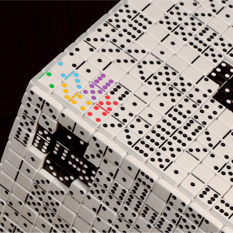
Sequence of domino fractions
A "domino-ified" Wallis-like product for pi
The Math section provides a much more detailed explanation of the adjustments I made to the Wallis product and the other math behind Metaphysics.
Dimensionality and Topology
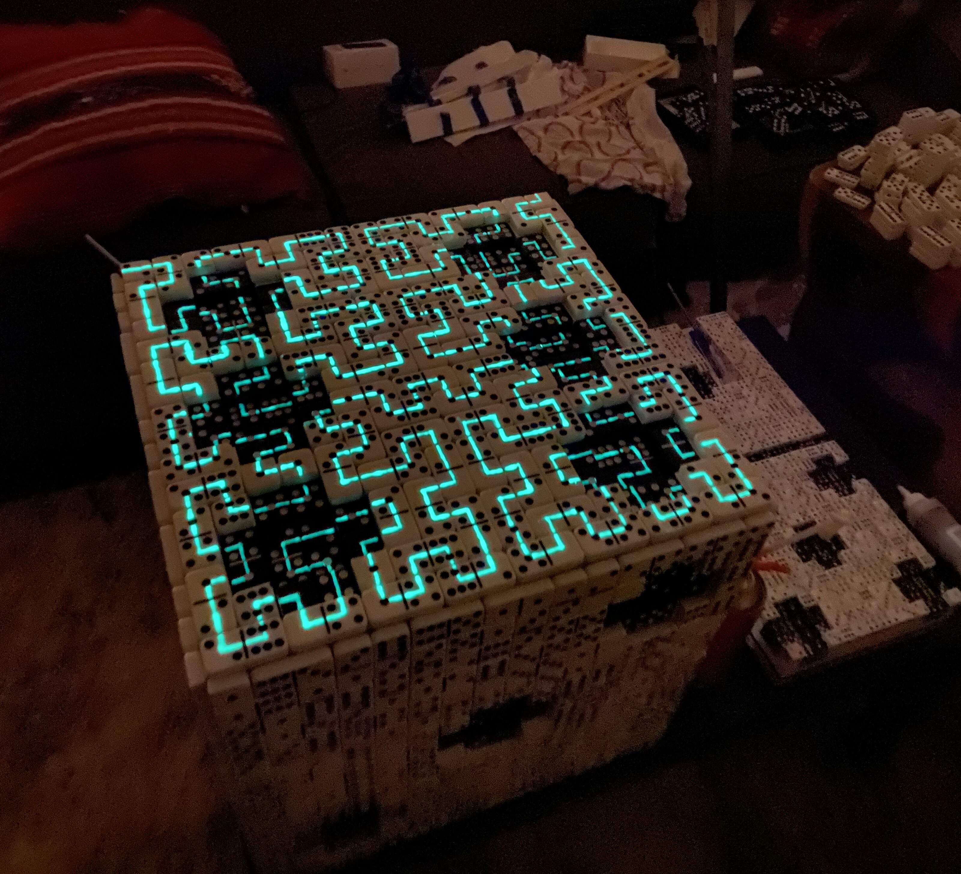
But there's even yet another pattern hiding in the dominoes, a pattern that only reveals itself in the dark.
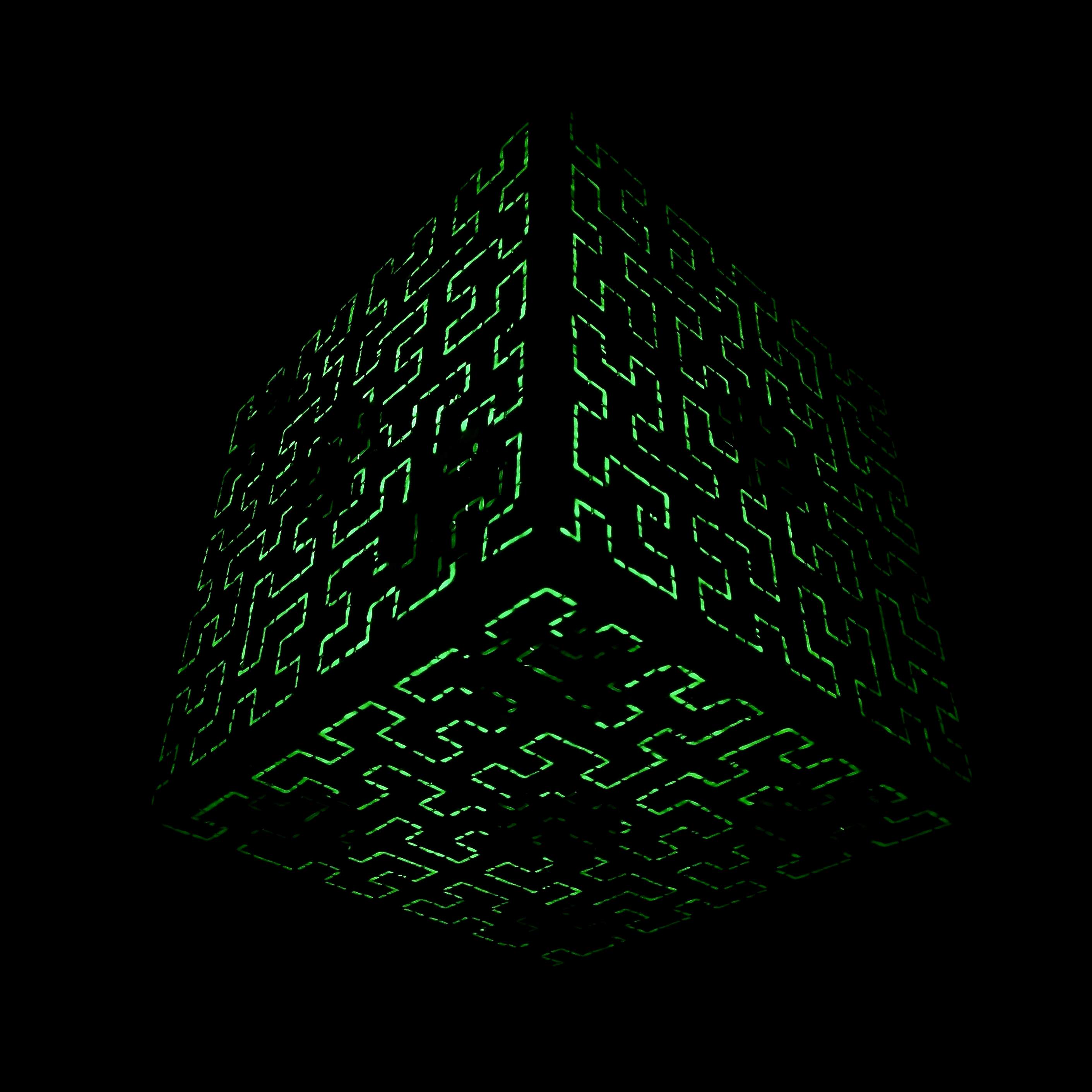
The die of dominoes in the dark!
A ghostly Hilbert curve
The die is covered with thin lines of glow in the dark paint, which can be charged quickly with an ultraviolet (or "black") light. These lines form a striking pattern: a single, unbroken line that never crosses itself and yet covers the entire surface of the die, not missing a single square.
Space Filling Curves
This is what's called a Hilbert curve, named after David Hilbert, one of the most influential mathematicians of the 20th century. A Hilbert curve is a type of "space filling curve", which — as the name suggests — is a curve that fills all of space. It's a fractal, defined iteratively.
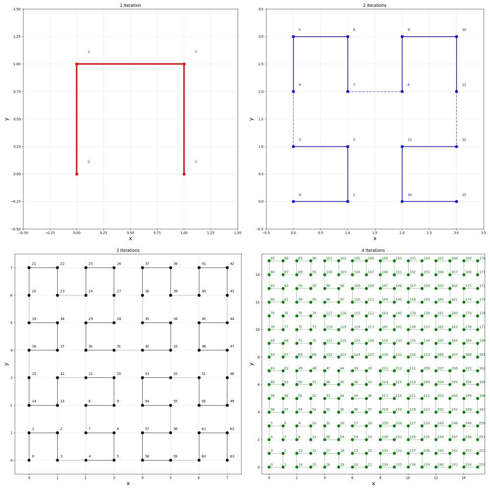
Four iterations of a (polygonal approximation to a) Hilbert curve
In the infinite limit, the Hilbert curve fills all of space
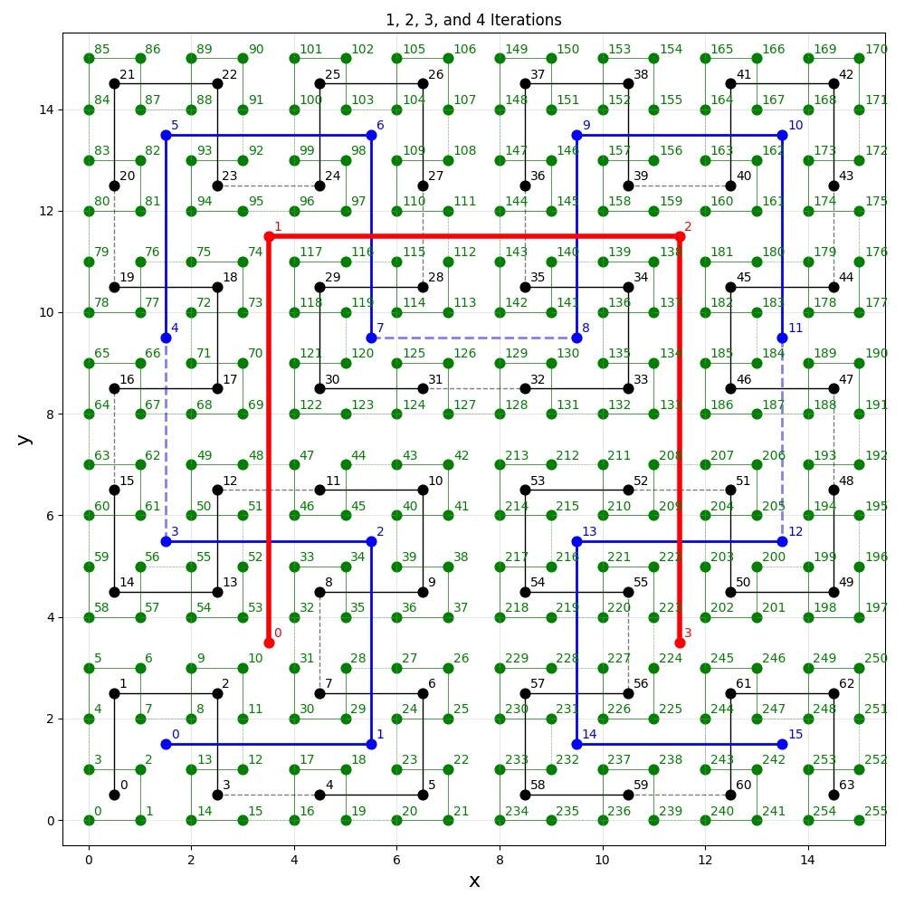
Four iterations overlaid
We start with a simple U shape, and with each iteration we make small copies of the starting shape, rotate them, and connect them together. In the infinite limit, a Hilbert curve reaches every single point in space. Rather magically, it takes a one dimensional line and bends it in such a way that it completely covers a two dimensional surface.
This may seem like an esoteric bit of math with no practical application, but that's not the case. Hilbert curves are extremely useful for encoding two dimensional objects in one dimension, in a "resolution independent" way.
Image Encoding
For example, they're often used to encode digital images, which must be displayed to a person in two dimensions on a screen, at many different resolutions (depending on the strength of the network connection). And yet digital images, like all digital data, must ultimately be encoded in one dimension as strings of bits — lines of 1s and 0s.
Somehow, a website (like this one!) must display images to a person like you in such a way that they "look the same" no matter what the resolution is. Because of this, the one dimensional encoding must have a very particular structure that maintains a kind of "locality" for pixels. This is exactly what Hilbert curves provide.
To make this more concrete, consider a simpler space filling curve: the "snake curve" that simply snakes back and forth across the image. The problem with the snake curve for encoding images is that, as the resolution changes, pixels "jump around" all over the image. A pixel that's on the left side at one resolution might end up on the right side at another resolution. This makes the image completely garbled, far from "looking the same" to the viewer.
Hilbert curves behave differently because of their fractal structure. As the resolution changes, pixels move only slightly, maintaining roughly the same position, which preserves the essential features of the image.
For an excellent, detailed explanation of Hilbert curves and how they can be used to encode digital images, check out this 3Blue1Brown video:
Why is this relevant to Metaphysics? Because, as I said at the top, the current sculptures are small models of much larger ones I plan to build in the future. We can think of the dice and (half) dominoes that constitute the sculptures as physical "pixels" or "bits": white and black squares or 1s and 0s. Larger sculptures are built at higher resolutions. So, it's necessary to encode the image of the die in a resolution independent way!
Circular Tiling
The Hilbert curve of dominoes is remarkable for another reason. When you play dominoes, you line them up end to end with matching numbers, forming an unbroken line called a domino train. That line can be bent in all sorts of ways, as long as the numbers stay connected; in fact, it can loop back on itself, forming a circular train. This Hilbert curve of dominoes is itself a train, and moreover a circular train!
Domino train (left) and circular domino train (right)
The trains can be "bent" as long as the numbers still match
In other words, the die is created from a giant, unbroken loop of dominoes, scrunched and squiggled in just the right way that it perfectly covers, or tiles, the surface of the cube. Amazingly, it runs through every single coordinate square of the surface, without ever crossing itself.
Such a surface is what mathematicians called topologically closed because it wraps around on itself. It's two dimensional, but unlike a flat plane it doesn't stretch out to infinity. On a topologically closed surface, a closed loop can cover every point.
This circular tiling echoes a long history in mathematics of "domino tiling", which includes famous results like the Aztec diamond and Arctic Circle theorems and infamous puzzles like the (gruesomely named) mutilated chessboard problem.
Typically, a domino tiling involves covering a chessboard-like region with unnumbered dominoes of different colors. The Metaphysics die of dominoes takes it a few steps further, tiling a cube (six "chessboards" stuck together) with numbered dominoes... in a Hilbert curve patterned circular train!
Making
Notes
There seems to be a long standing cultural norm in both science and art to show only the final product of one's efforts. Why is this the case? I can only guess, but I'll point to several possible factors.
Perhaps presenters don't want to waste their audiences' time and assume those audiences aren't interested in anything other than the final product. Perhaps they don't share much information about process and mistakes made along the way because historically it hasn't been practical to do so. Perhaps they deliberately hide the "how" and "why" so audiences will be amazed by the mystery and enabled by the vagueness to read whatever they like into the work.
Whatever the reasons may be, I'm thrilled to live in a time when this is changing. Today, enabled by the internet, people are sharing more information than ever before in human history. Often, they're completely pulling back the curtain to show every step of their process and thinking. While I too am tempted to hide the evidence of how and why I made my work, for sake of the "wow" it can induce, I'm even more excited to show the world the view from behind the scenes.
That's what this section is about: showing you, the viewer, the how and why with minimal curation. Perhaps this a level of detail too excruciating for most, but I hope for some it serves as a curious record of one man's creative process.
Most of all, I hope you see my mistakes and missteps in broad daylight. These bumps in the road are the thrill of creation itself! No matter how polished and pristine the final product may be, the road to get there is never smooth, nor would I ever want it to be. I hope you can be as entertained and intrigued as I am, looking back through the many dead ends I encountered.
In Full, Unedited
Here are the notes I made while making Metaphysics — in full and unedited:
Complete, unedited notes
And here is a spreadsheet I used before switching to writing code, which proved to be much more flexible:
For both documents, the exporting process messed up some of the formatting, but all of the content is there. I'm happy to share an editable version of the spreadsheet — just contact me if you'd like it.
Snippets
The first note I made about Metaphysics (just a vague idea without a title at the time) was on April 27, 2021. It included little more than this hilariously basic drawing:
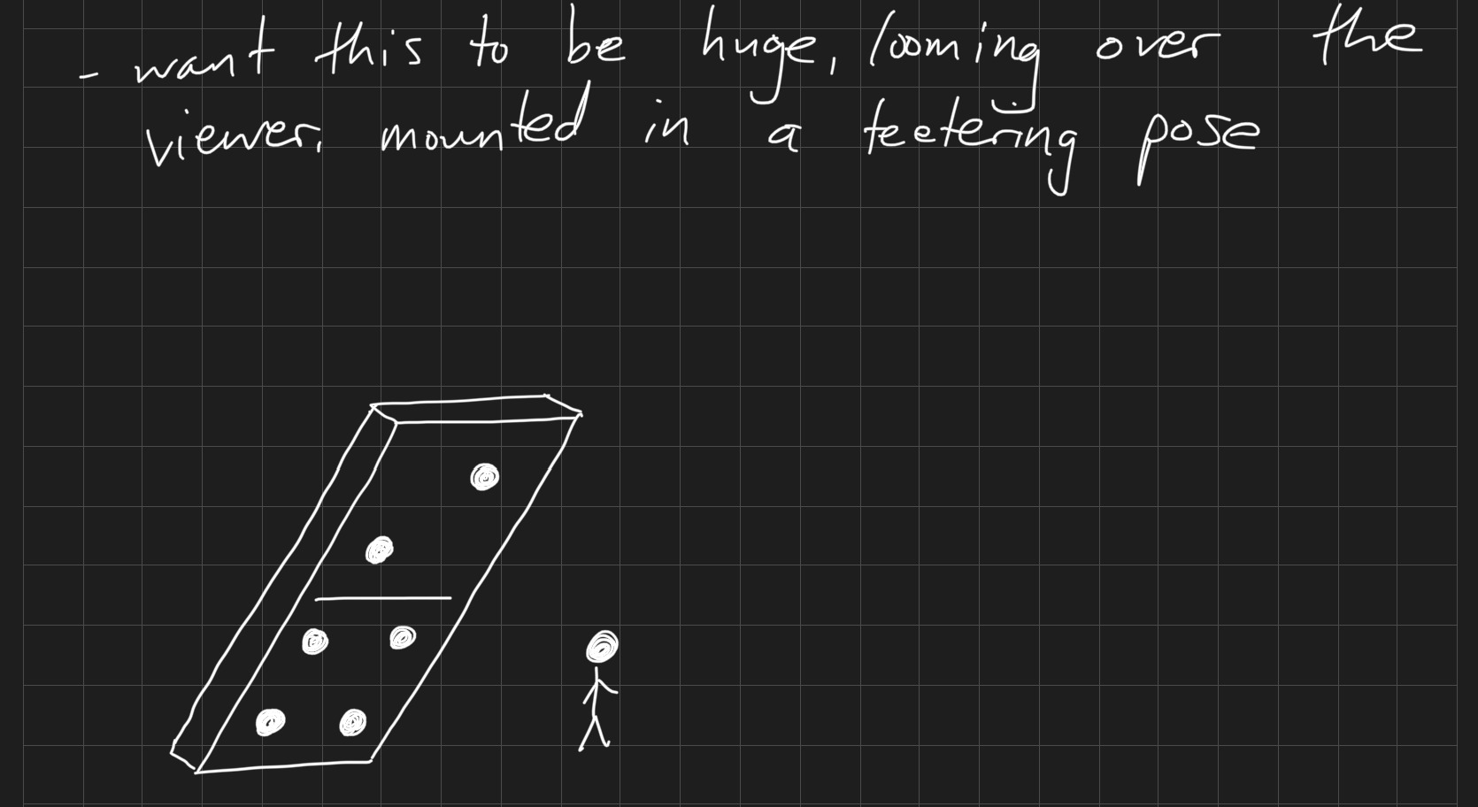
My first drawing of the domino of dice
It started off extremely primitive!
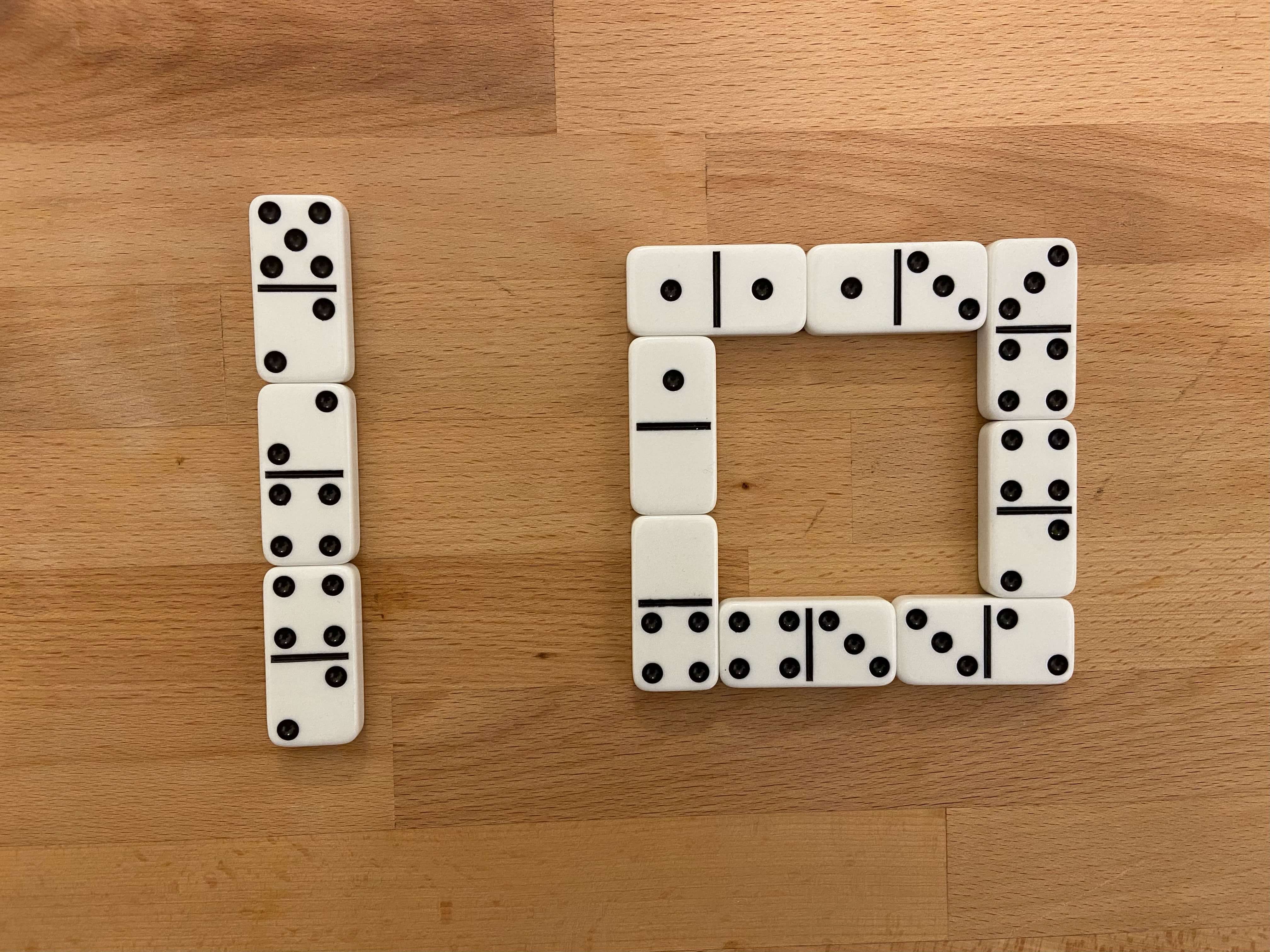
A friend of mine helpfully encouraged me to start by building small scale models of the sculptures. I began by sorting out how many dice I would need to make the domino of dice:
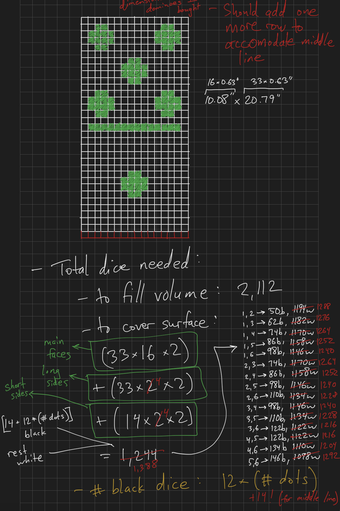
Figuring out how many dice I'd need
Before switching to writing code, I made extensive use of a spreadsheet. Here I was using it to calculate how many dice and dominoes I would need (and how much they might cost) for sculptures of different scales:
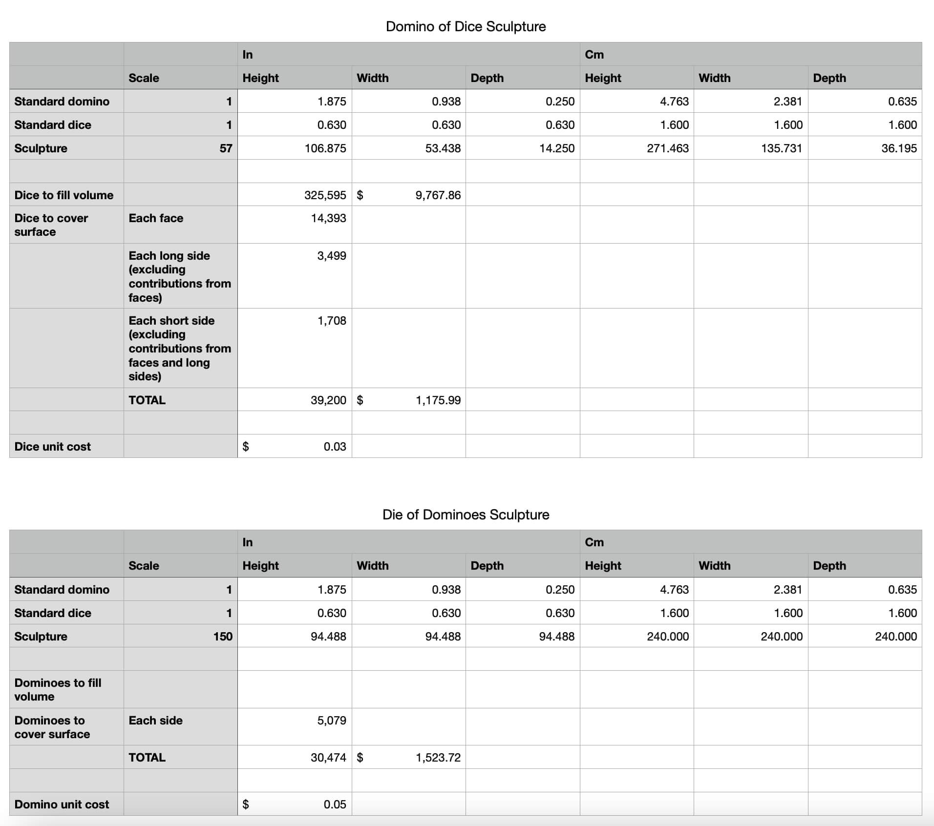
Spreadsheet calculations
I also used the spreadsheet to determine which dominoes would be within which dots (on the die of dominoes). This became extraordinarily complicated, which ultimately made me switch to writing code.
Spreadsheet calcuations and diagrams
I went through many iterations of how to make the die of dominoes, which included lots of checking what was possible:
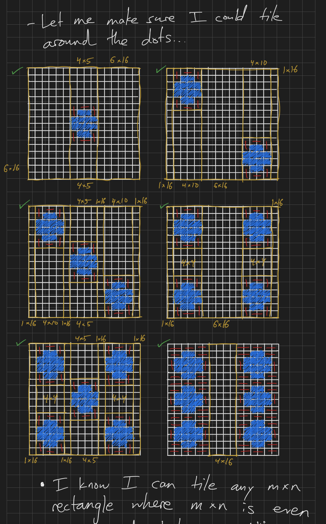
Making sure it's possible to tile around the dots
Here, I'm trying to figure out how to wrap a Hilbert curve over the full surface of the die of dominoes, looping back on itself:
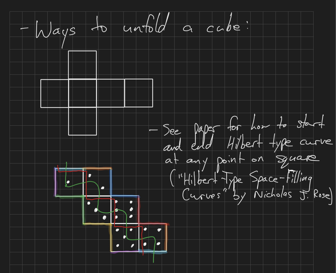
Exploring ways of unfolding a cube
Much of this project was mathematical in nature, but mathematics can be visual as much as it can be notational. Here, I inadvertently showed in a visual way that what I was hoping to do was simply impossible:
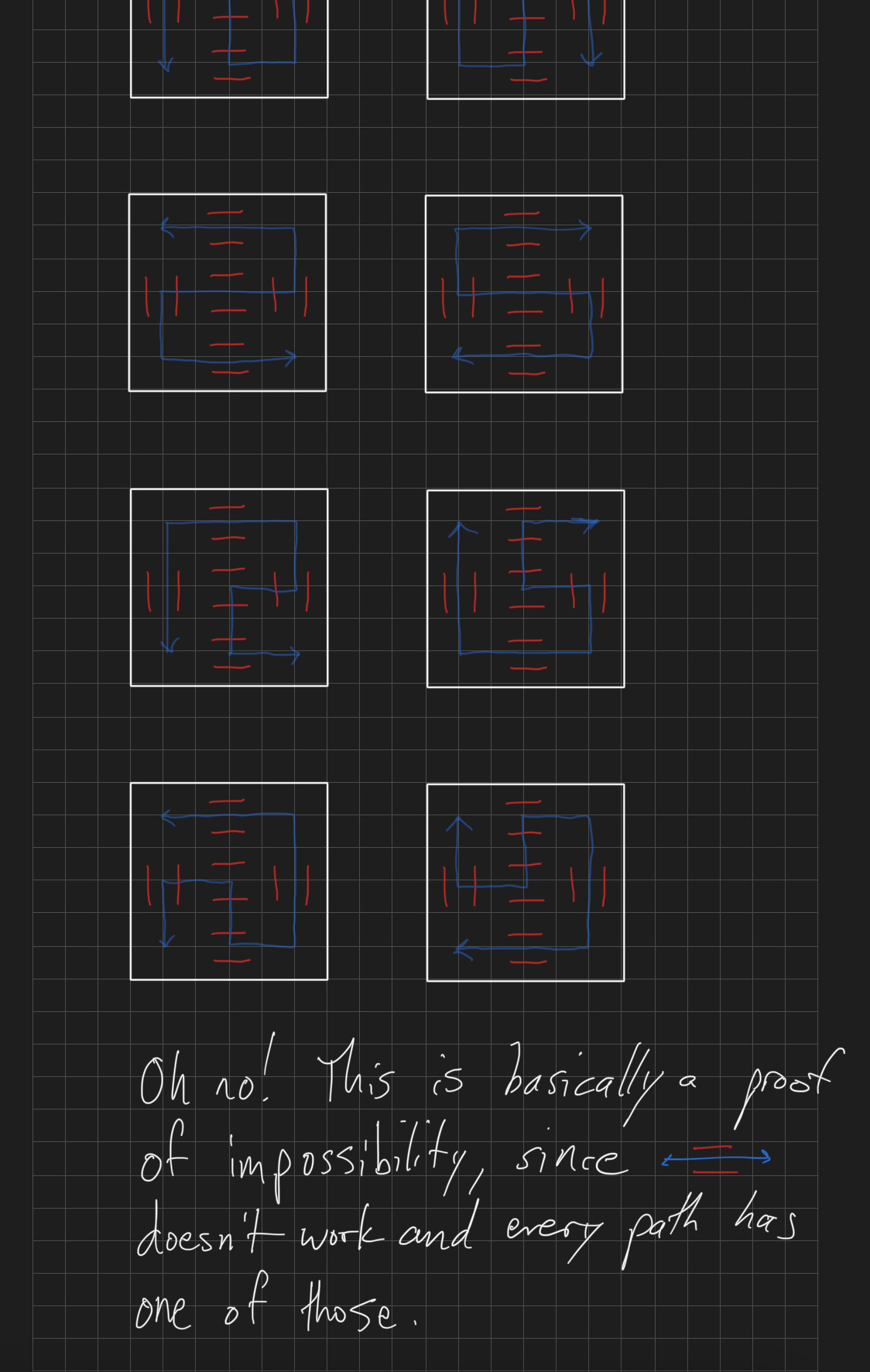
A visual proof of impossibility!
"Oh no!"
I spent so much time trying to find dot like shapes in domino tilings based on Hilbert curves. Amazingly, these shapes exist, but unfortunately they don't exist in the right positions to serve as dots on a die.
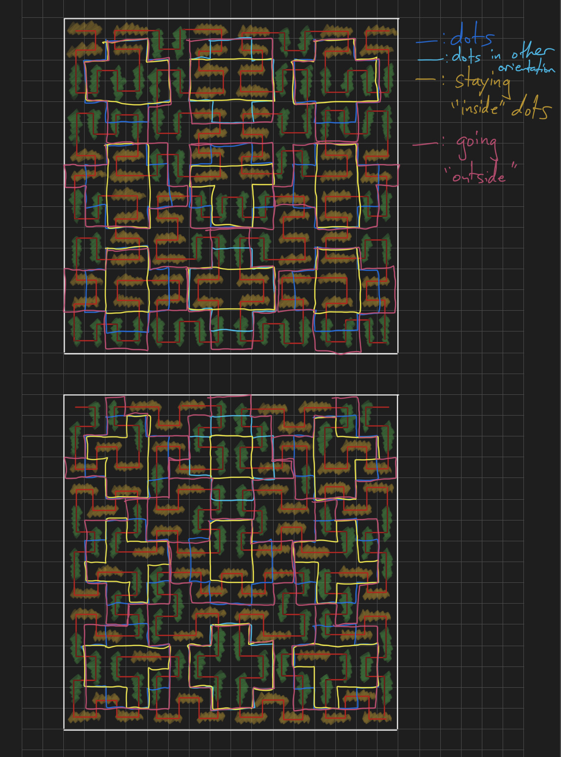
Trying to find dots within a Hilbert curve
Much of my effort went toward sorting out which questions to ask. Here, I finally consolidated several key questions about domino sequences I could then try to answer:
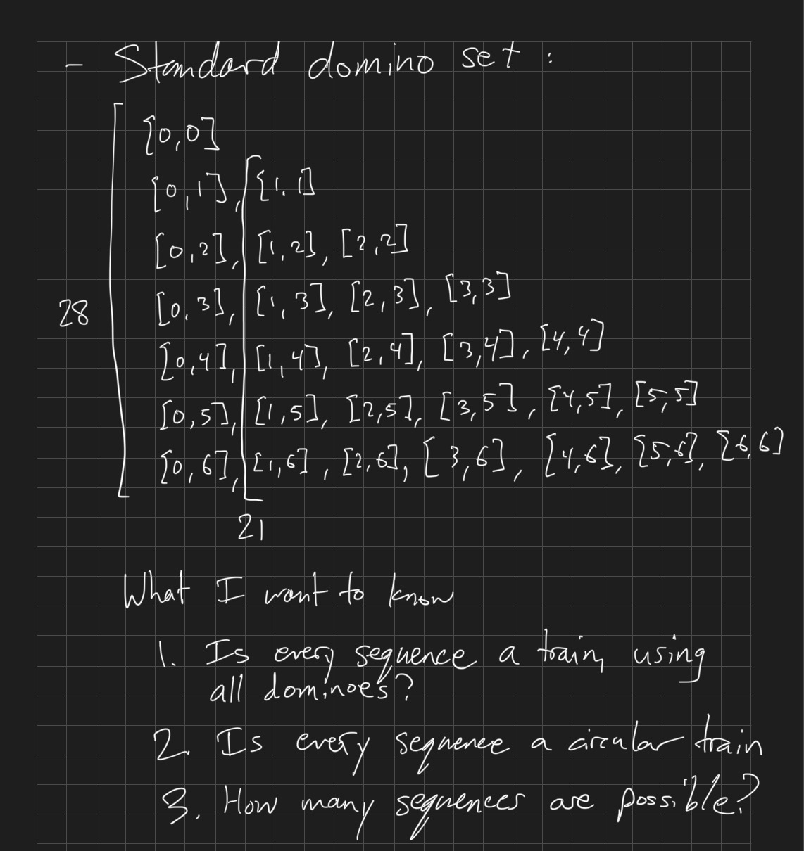
Deciding what I needed to know
An amusing example of the frustrating process of inventing a language for the things you're trying to but don't yet understand:
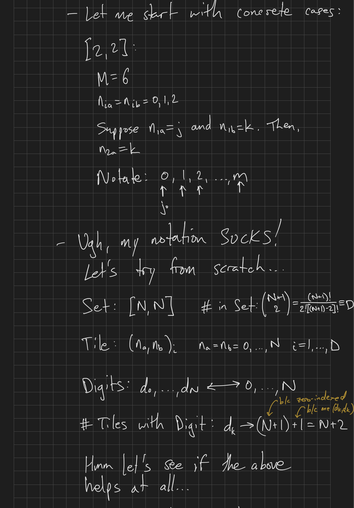
Getting confused
"Ugh, my notation SUCKS!"
One of countless dead ends:
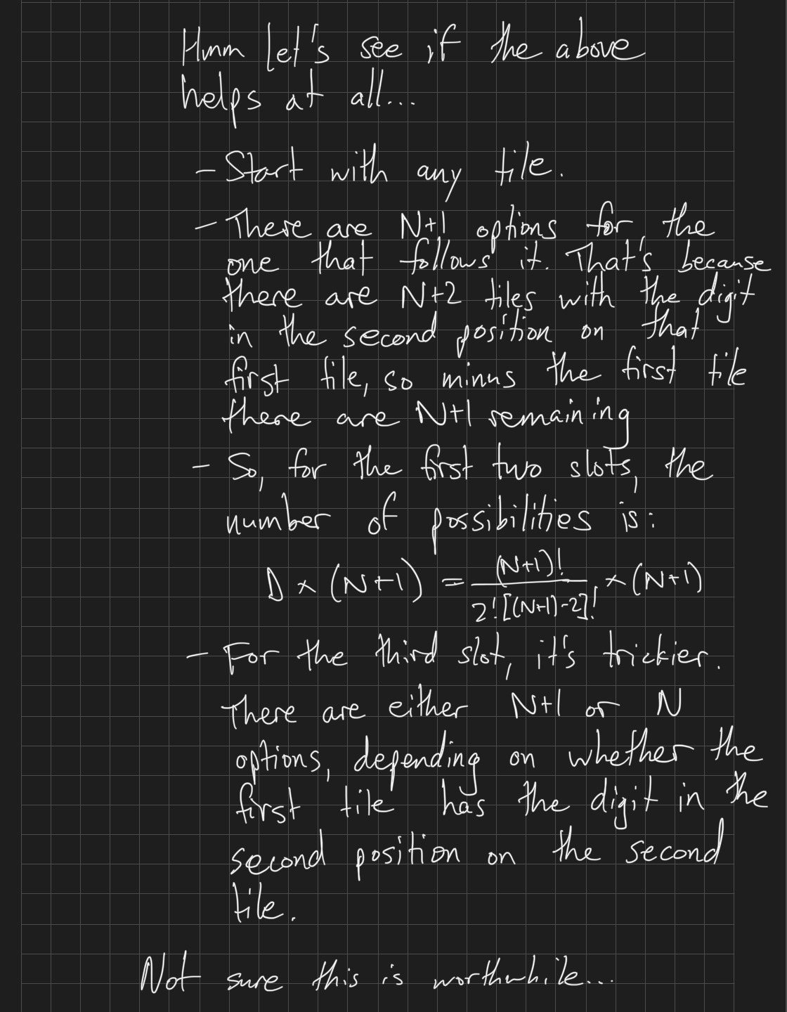
Looking down rabbit holes
"Not sure this is worthwhile..."
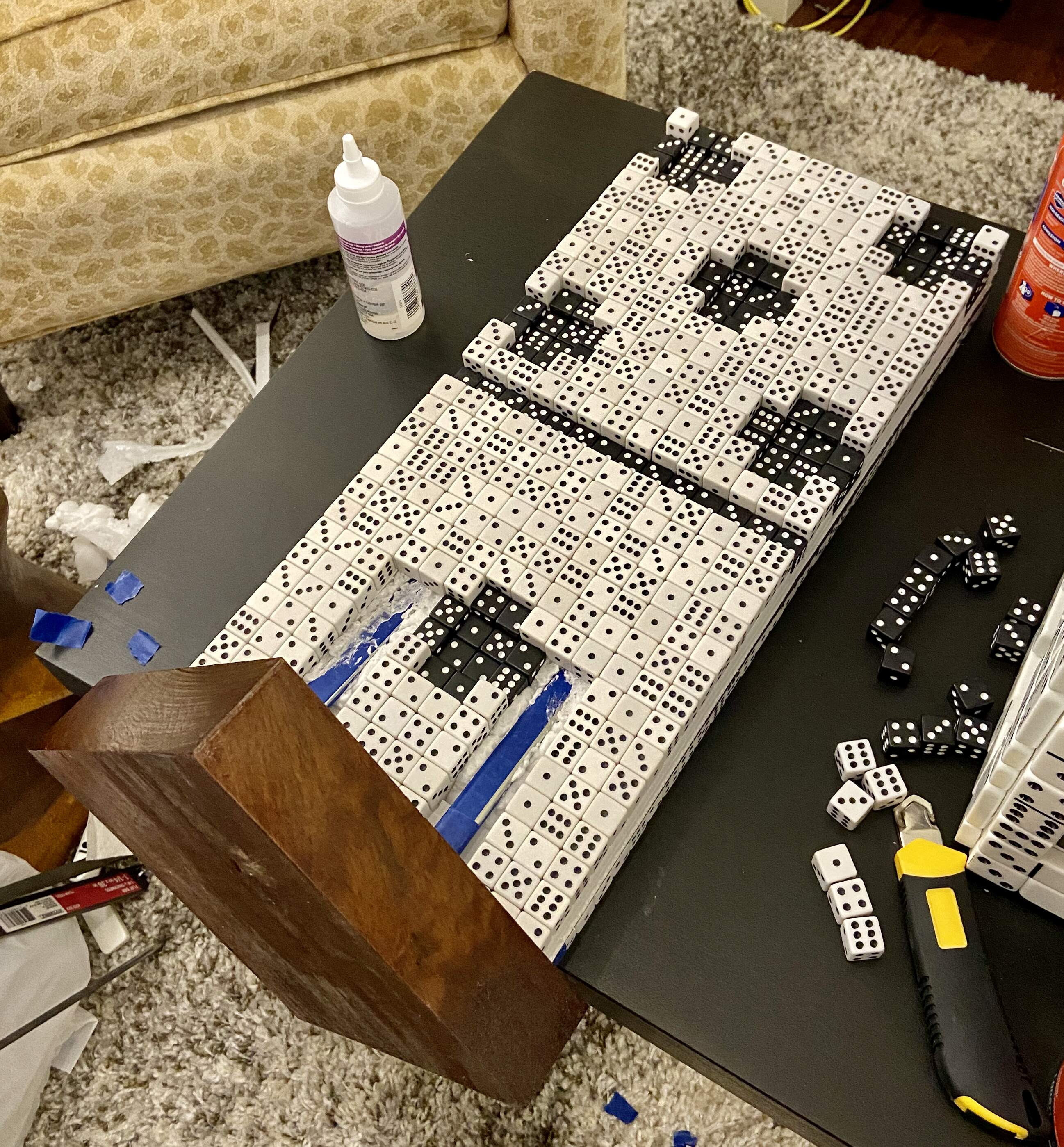
Below is my initial plan for how to build the domino of dice. This turned out to be quite difficult to get right, as it involved creating a substructure beneath the dice that ideally would intersect with as few of them as possible. (Any dice the substructure intersected with were dice I'd have to slice... which I knew would be difficult to do accurately.)
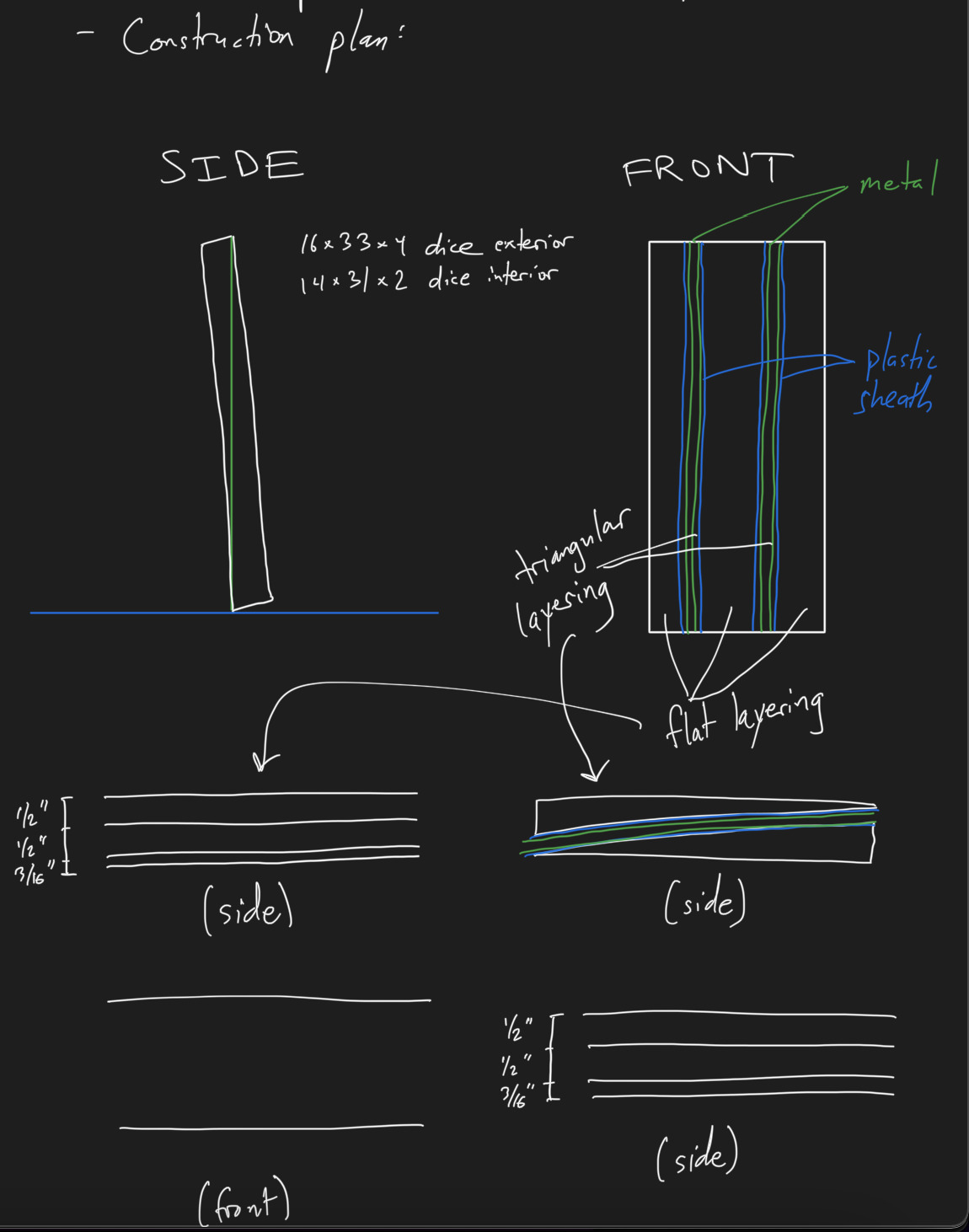
Construction plan
Even finding simple angles could be a decent amount of work!
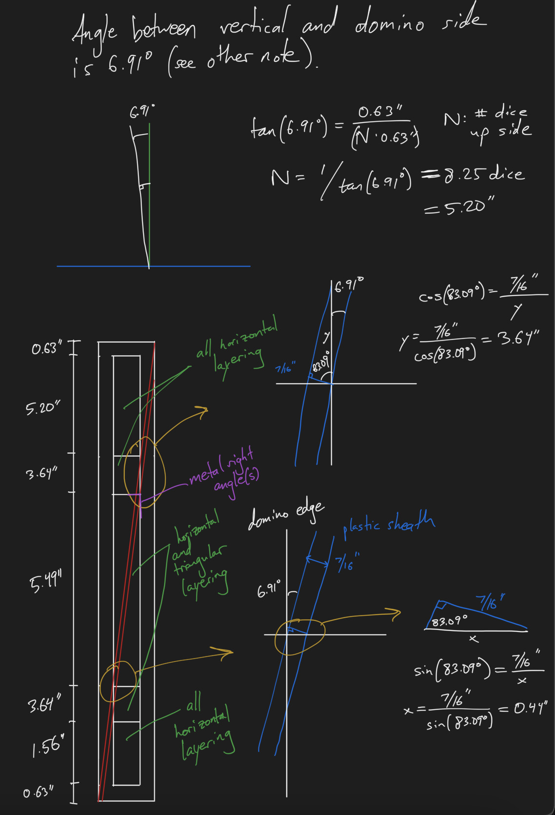
Finding various angles
An example of uncovering a wrong assumption, which is the best of feelings:
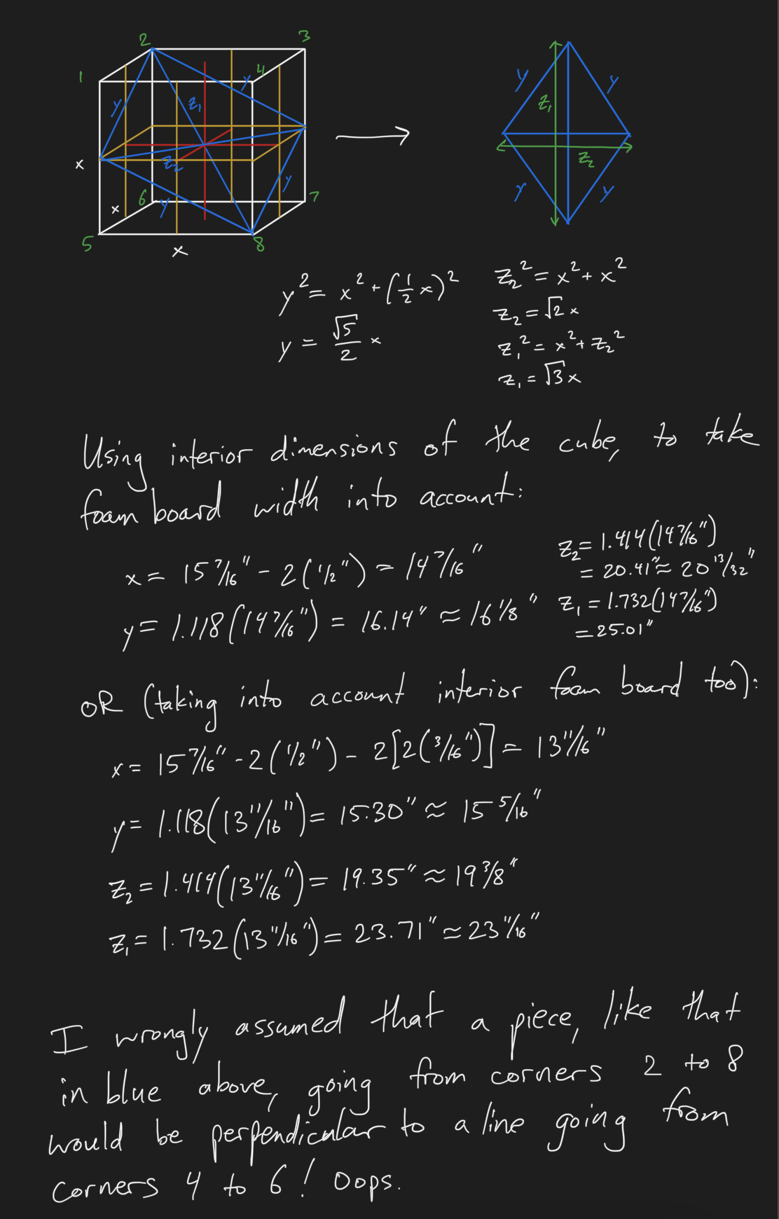
A wrong assumption
"Oops"
This looks like a high school geometry exercise! That trigonometry sure came in handy.
Trigonometry
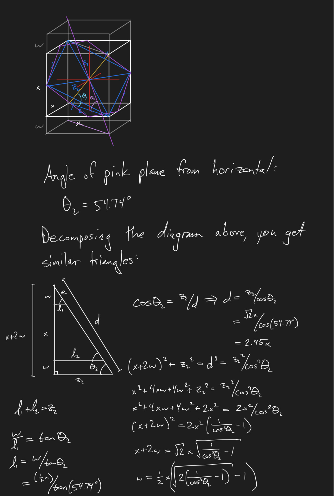
One of the joys of math is how it can surprise you and change your intuitions. Here's a great example, where I unknowingly drew a diagram dramatically out of proportion but then realized from my calculations that it was in fact a regular hexagon. Drawing is imprecise, but equations never lie. (In my excitement, I apparently forgot how to spell "whoa"!)
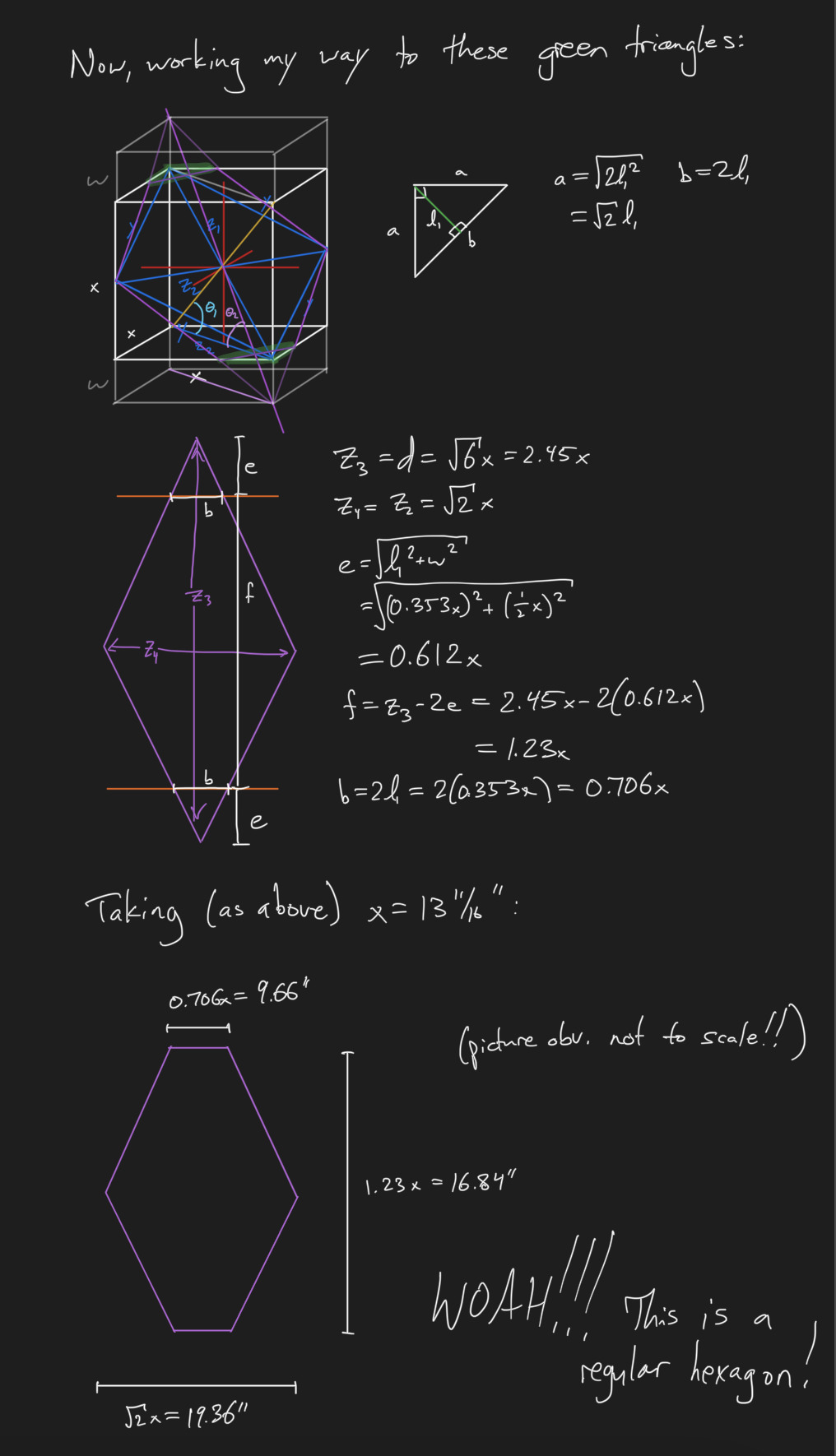
A regular hexagon!
"WOAH!!!" (sic)
I went through all sorts of variations on "domino encodings", starting with infinite sums of fractions like these:
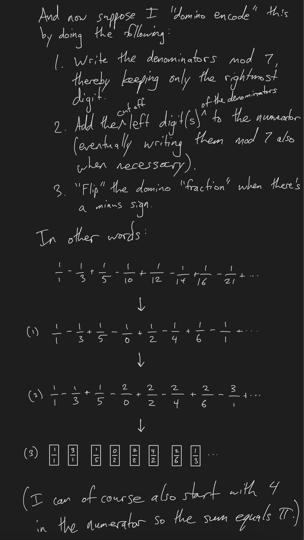
Domino encoding
Later, I tried adapting the Wallis product, which proved extremely fruitful:
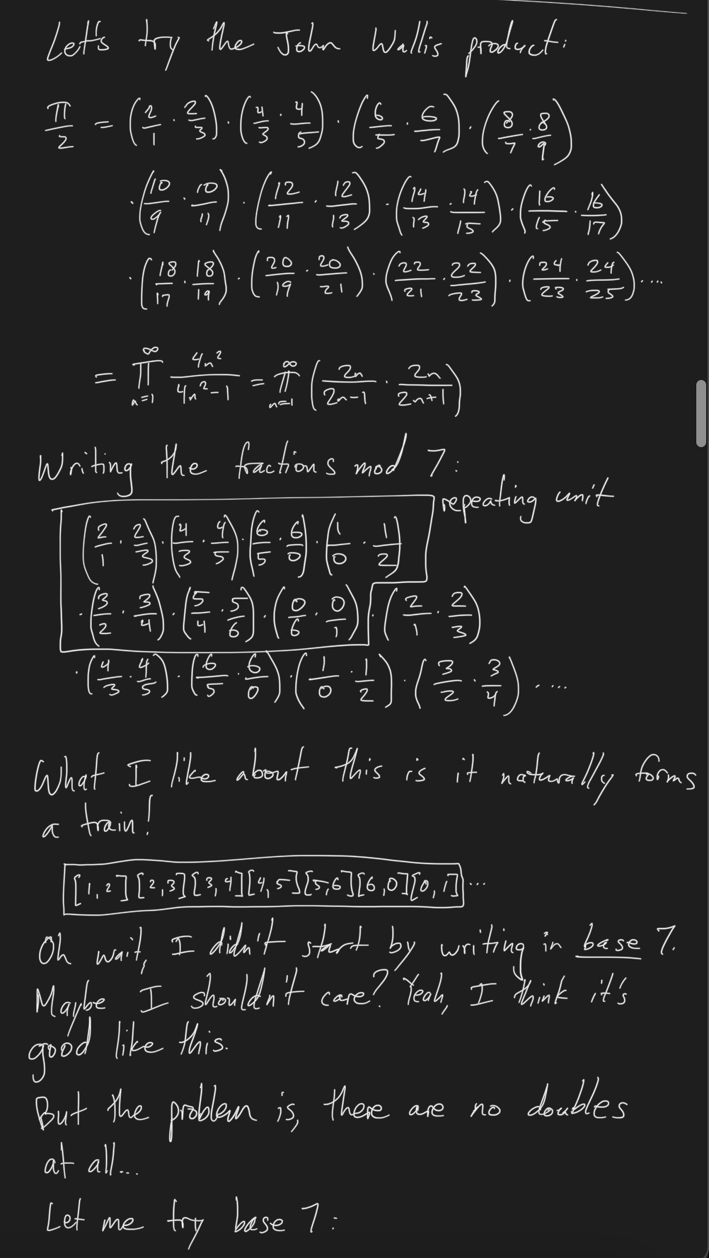
Adapting the Wallis product
At some point, my code became complex enough that I needed to diagram how all the quantities and functions fit together:
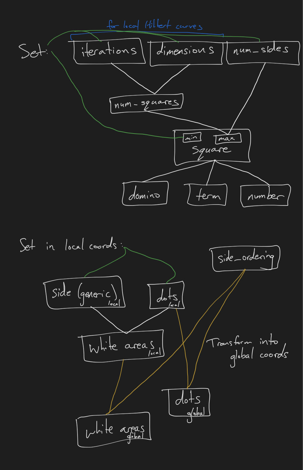
Code system diagram
Images and Videos
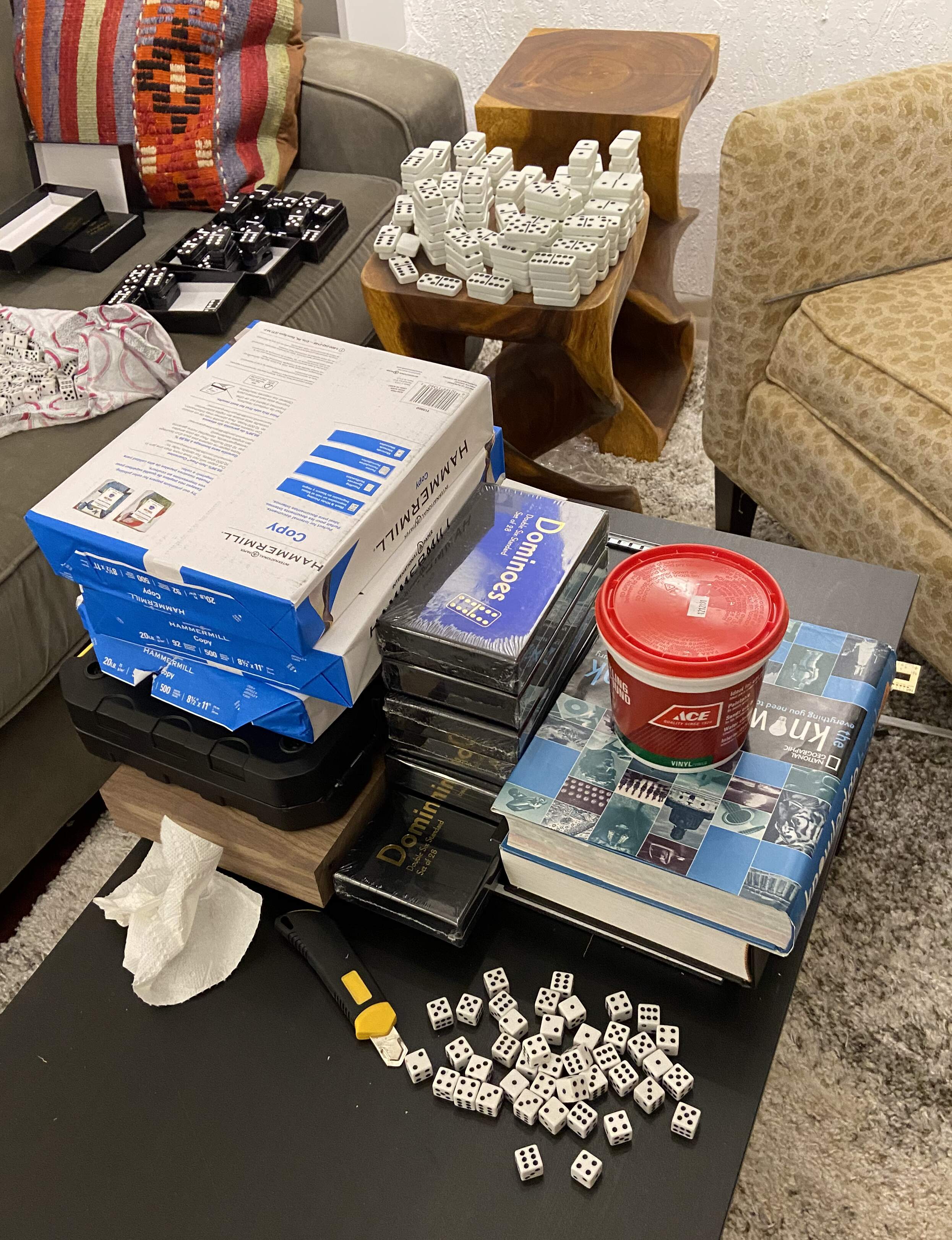
I began by purchasing 868 dominoes and 1,400 dice, and posting on social media that I did. Having the raw materials and telling people you're going to do something with them is a great way to self motivate!
My Instagram story at the start of construction
October 21, 2021
I started by trying many different ways of making a dot for the domino of dice, to see which one felt most accurate:
Experiments with different types of dots
For the domino of dice
I then made a crude block domino to see how that would look:
Block of dice in domino shape
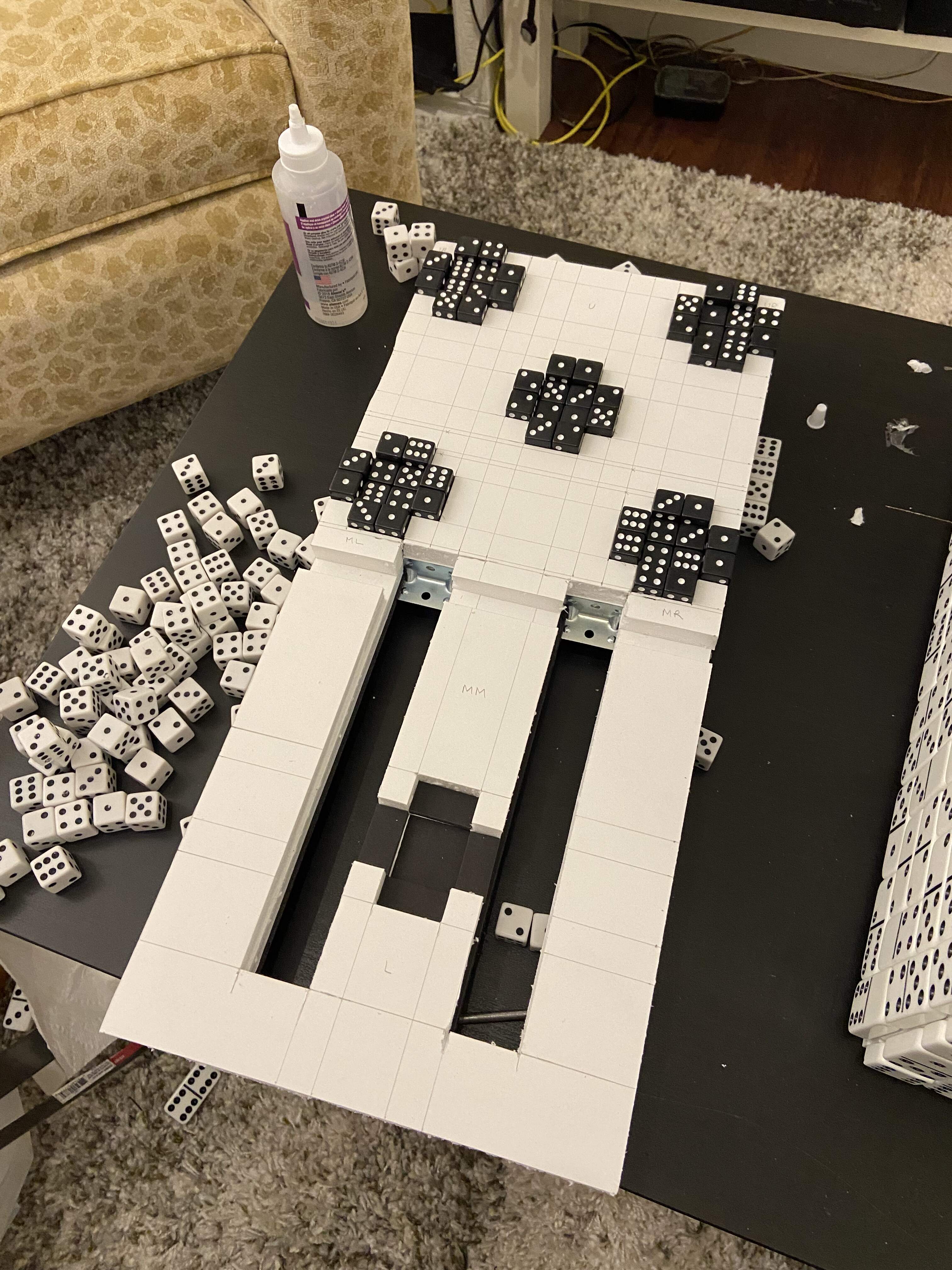
After tons of effort, I finally settled on using angle braces to let internal supports prop up the domino:
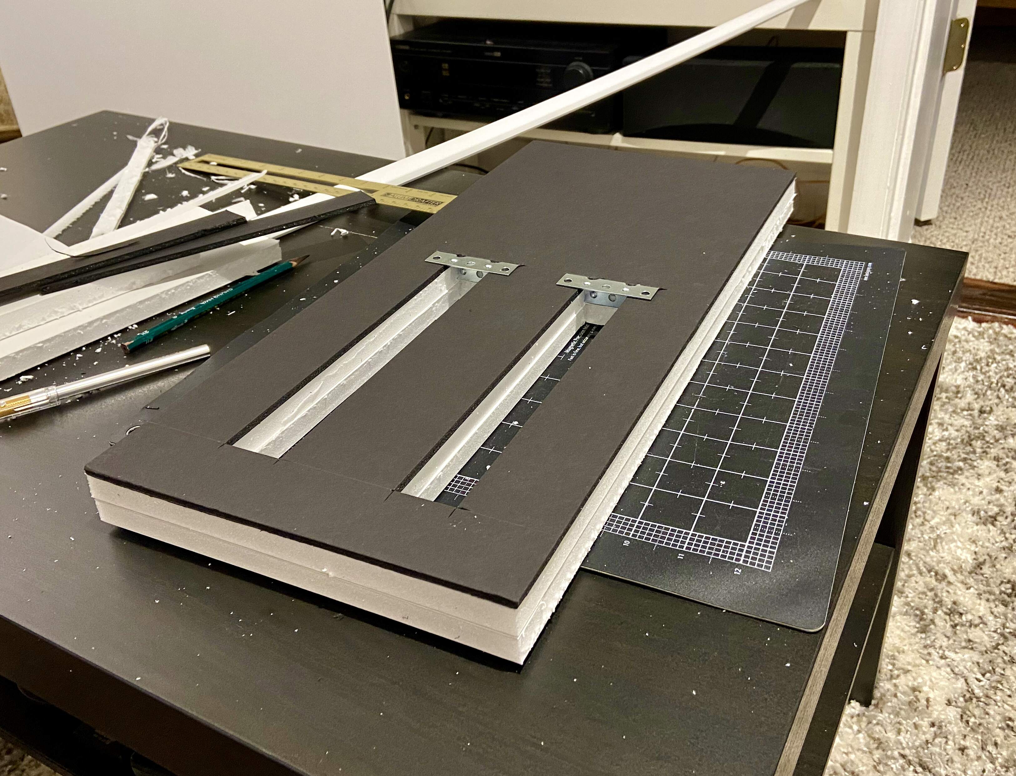
Angle braces to support the domino of dice
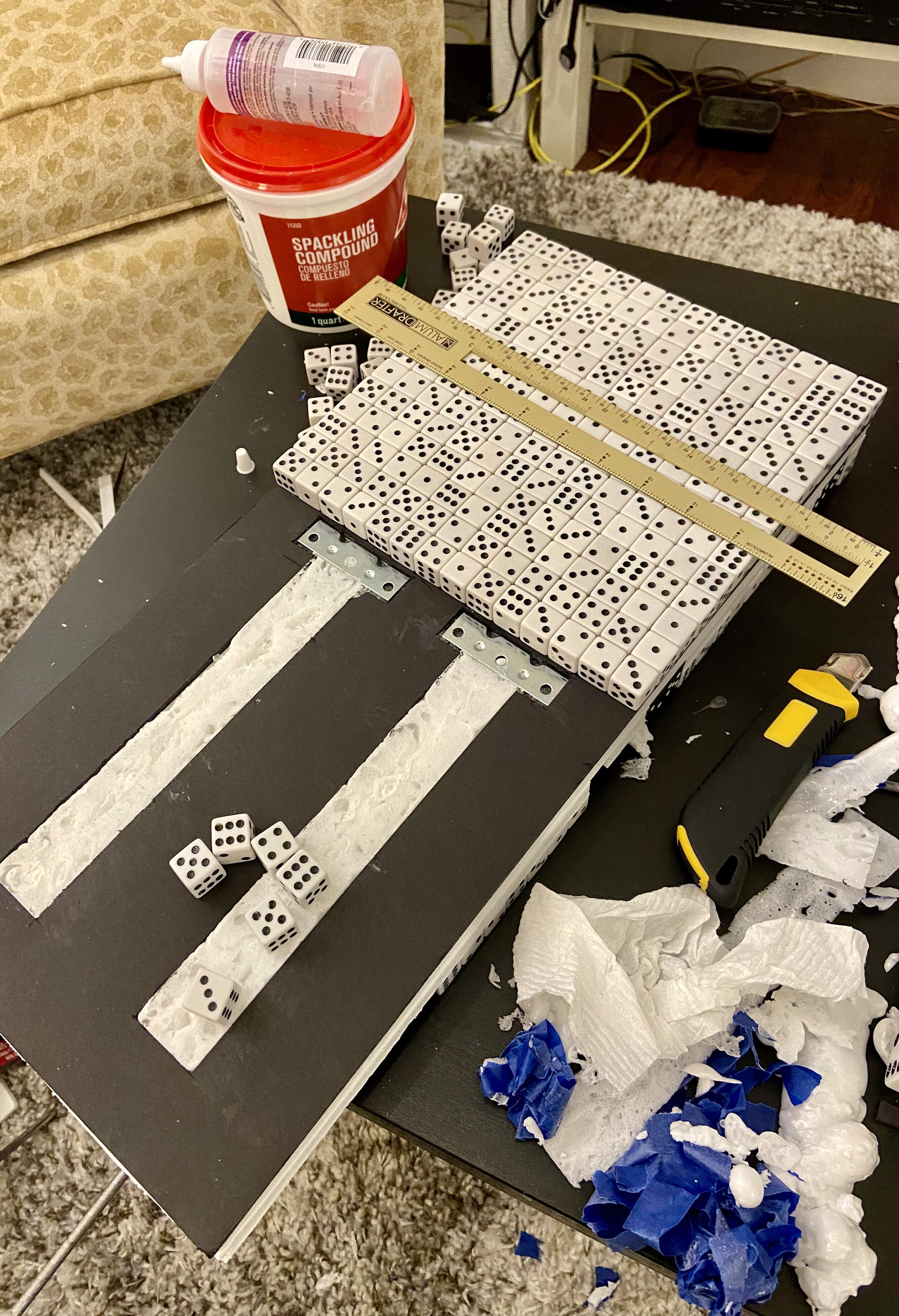
Here I was checking that the length of the foam board I cut matched the right number of dice:
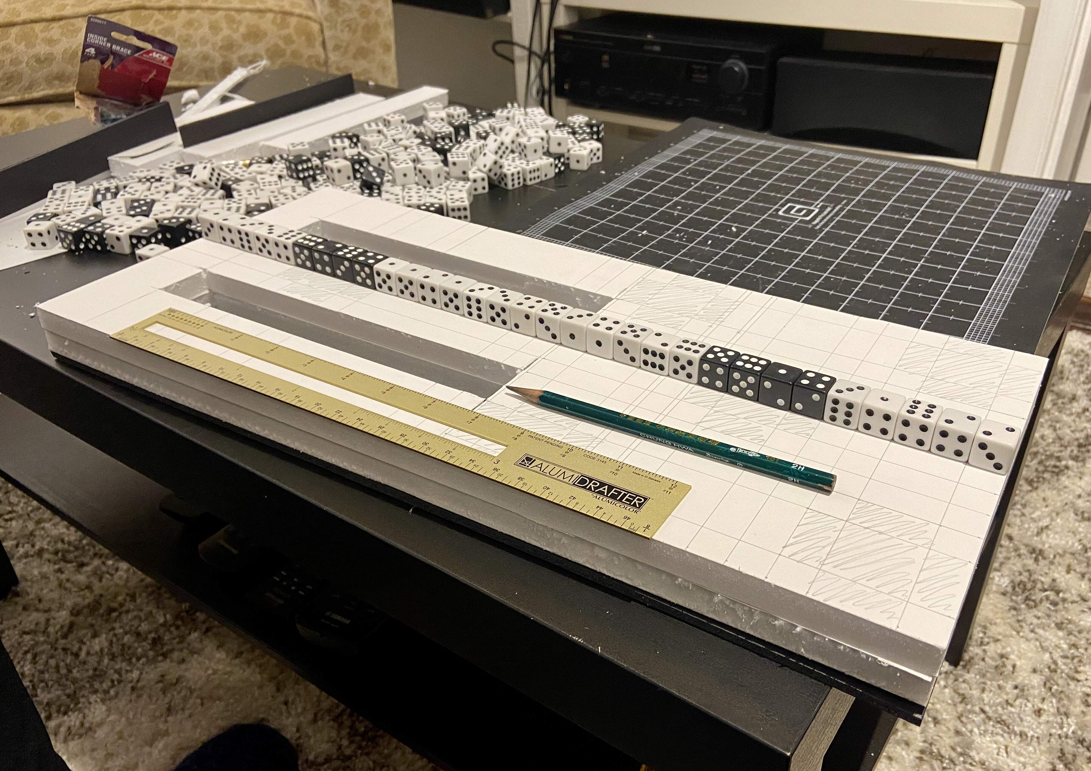
Checking that the length is correct
Here's most of the foam board structure for the domino of dice:
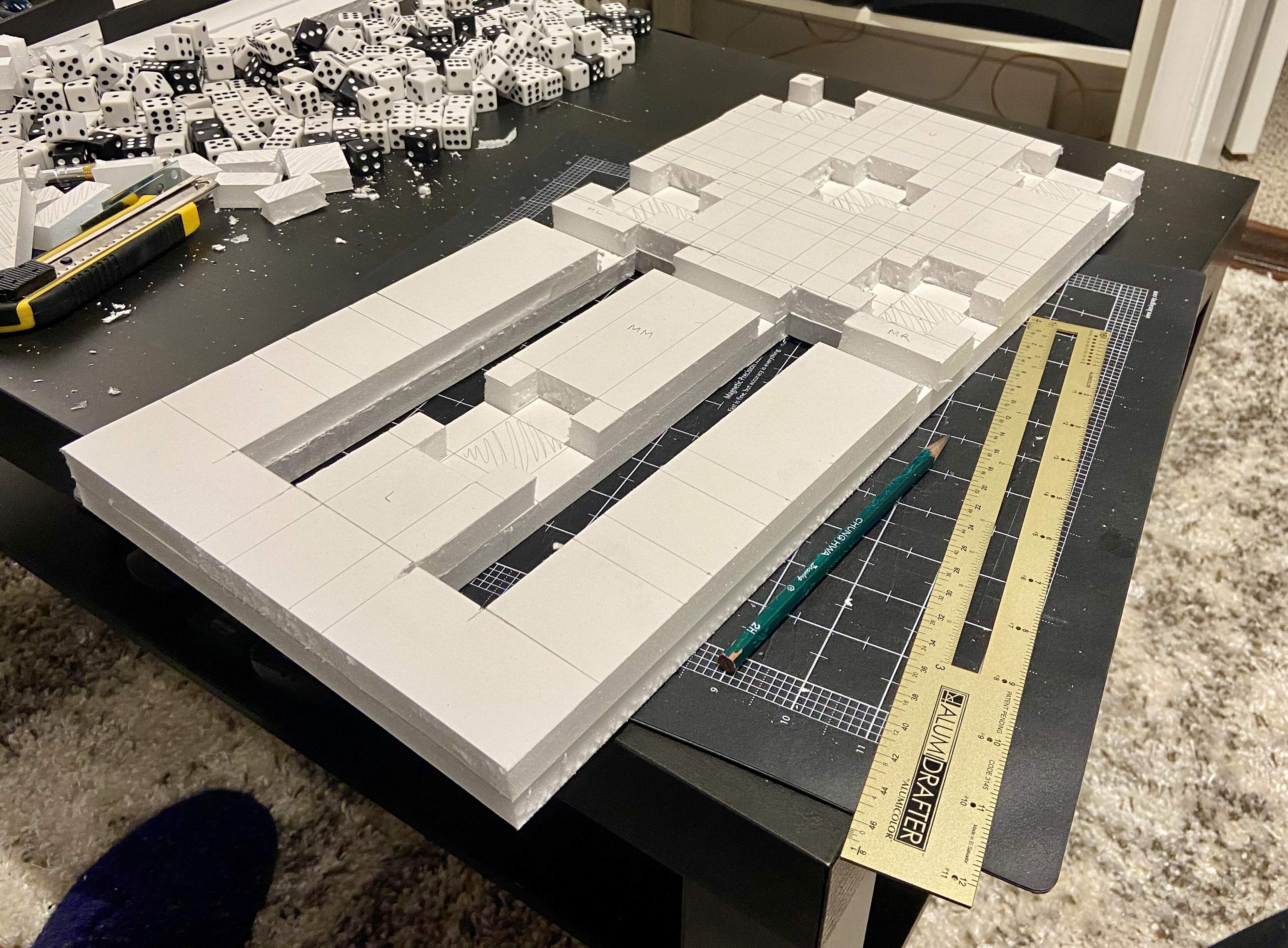
Foam board structure
I carefully followed notes I'd made to create a Hilbert curve pattern of dominoes. This is when I realized it didn't exactly jump out at the viewer! And that inspired me to find a way to make the pattern more apparent, which ultimately led me to use glow in the dark paint. Great ideas often come from wrong turns!
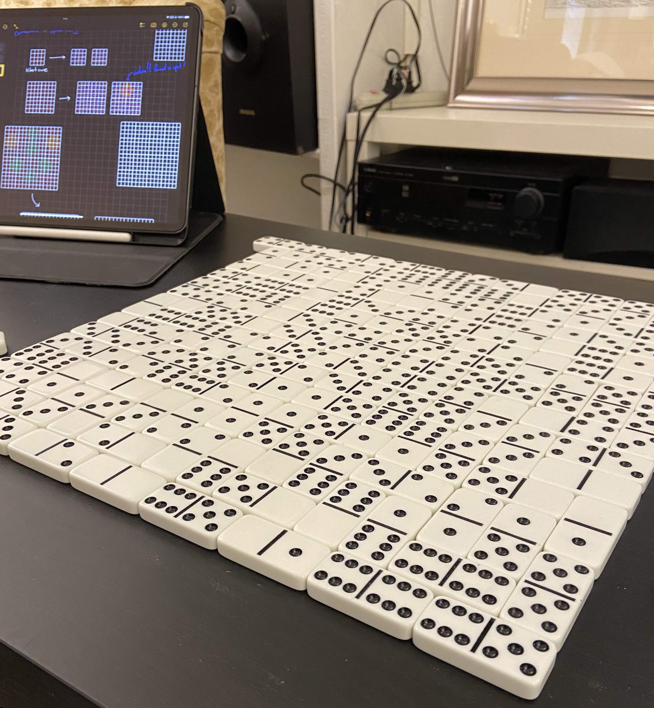
Making a Hilbert curve of dominoes
Using iPad drawings as a guide
Similar to the tests I did for the domino of dice, I experimented with different types of dot structures for the die of dominoes.
Experiments with different types of dots
For the die of dominoes
The die began as a simple blank cube. It was surprisingly difficult to get the dimensions of the cube exact enough, due to slight warping in the foam board.
Blank foam board cube
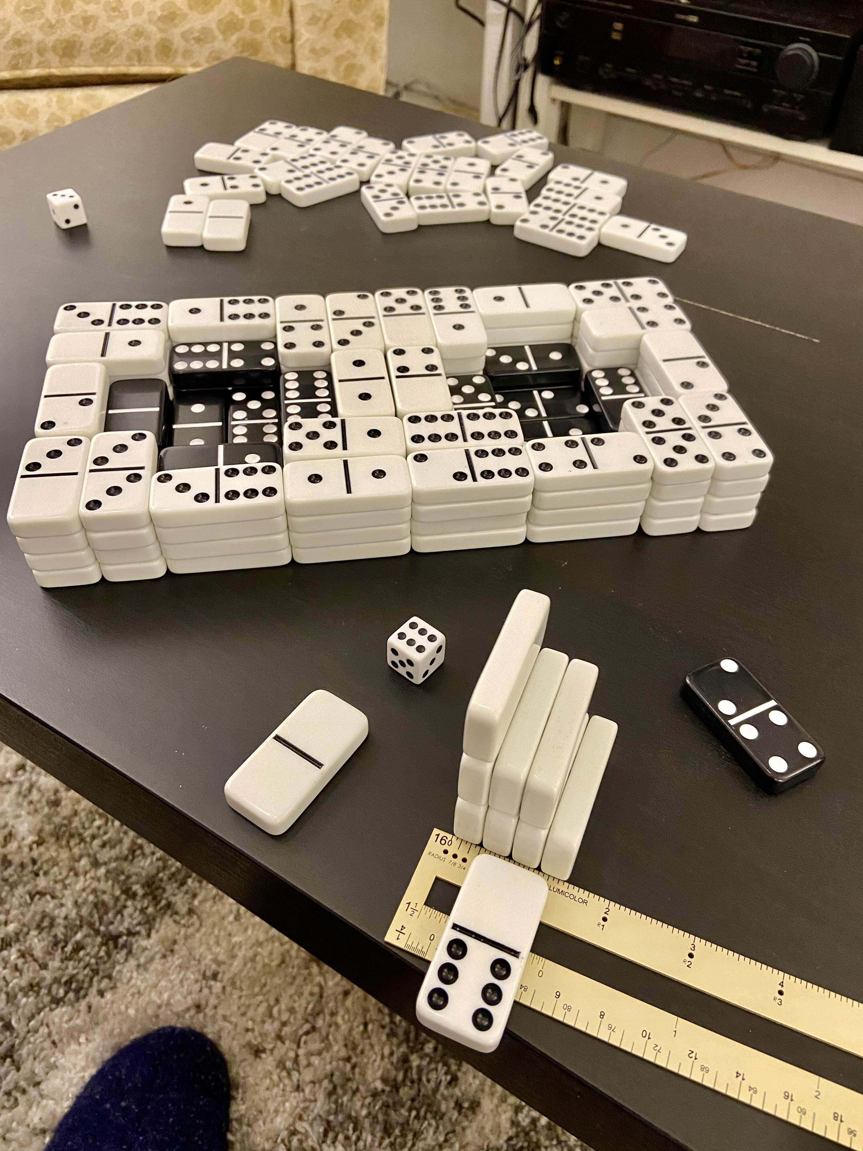
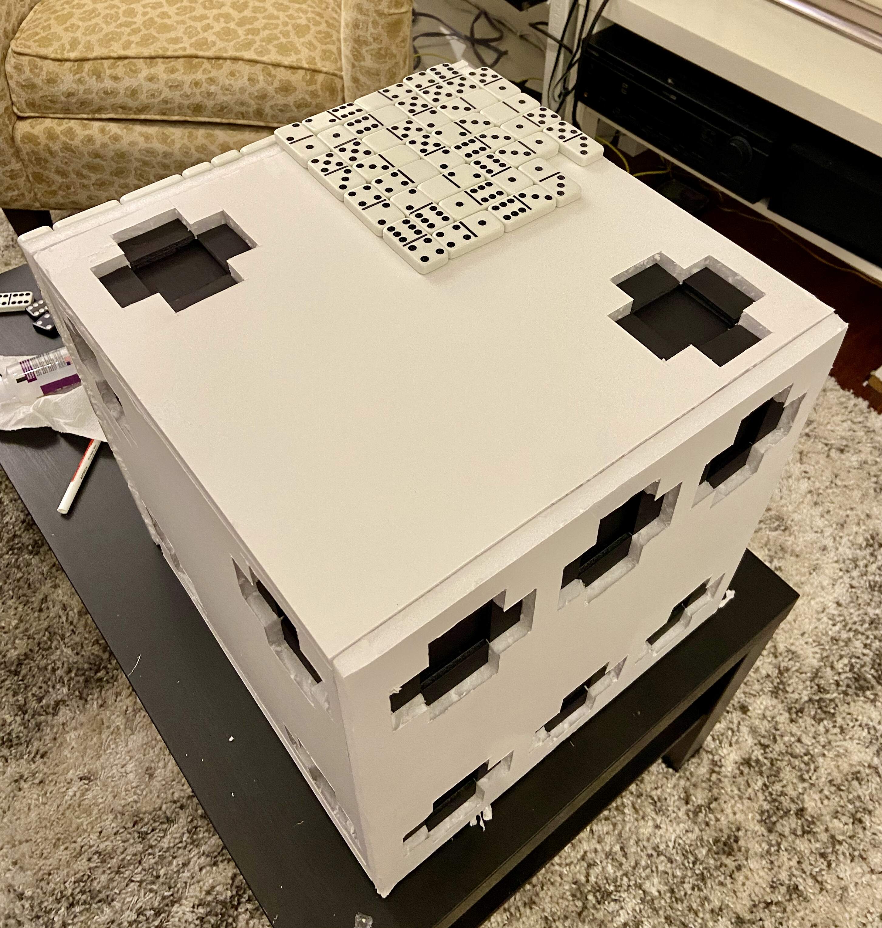
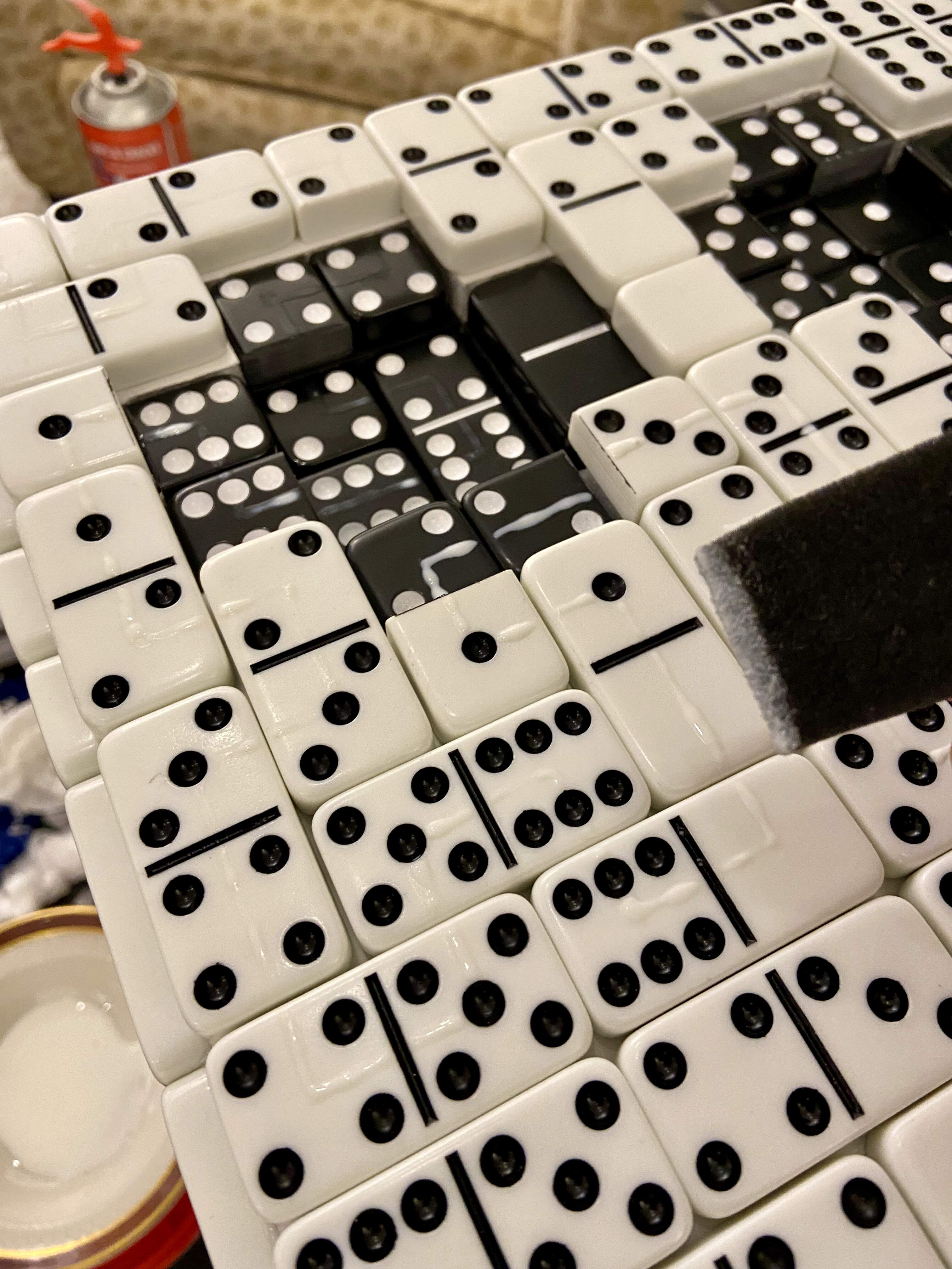
It was so exciting to see the dots made out of dominoes for the first time:
Partial covering to test dots
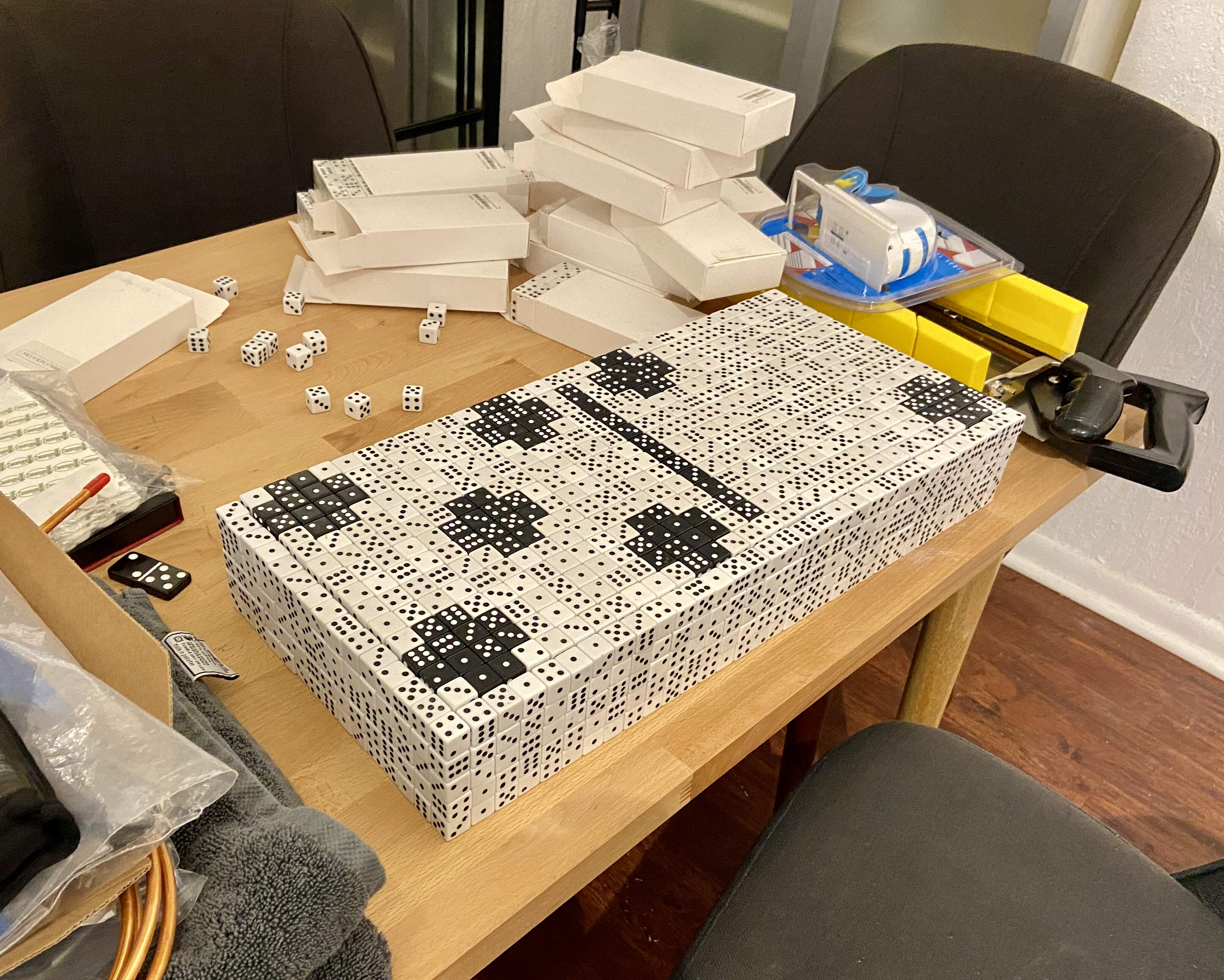
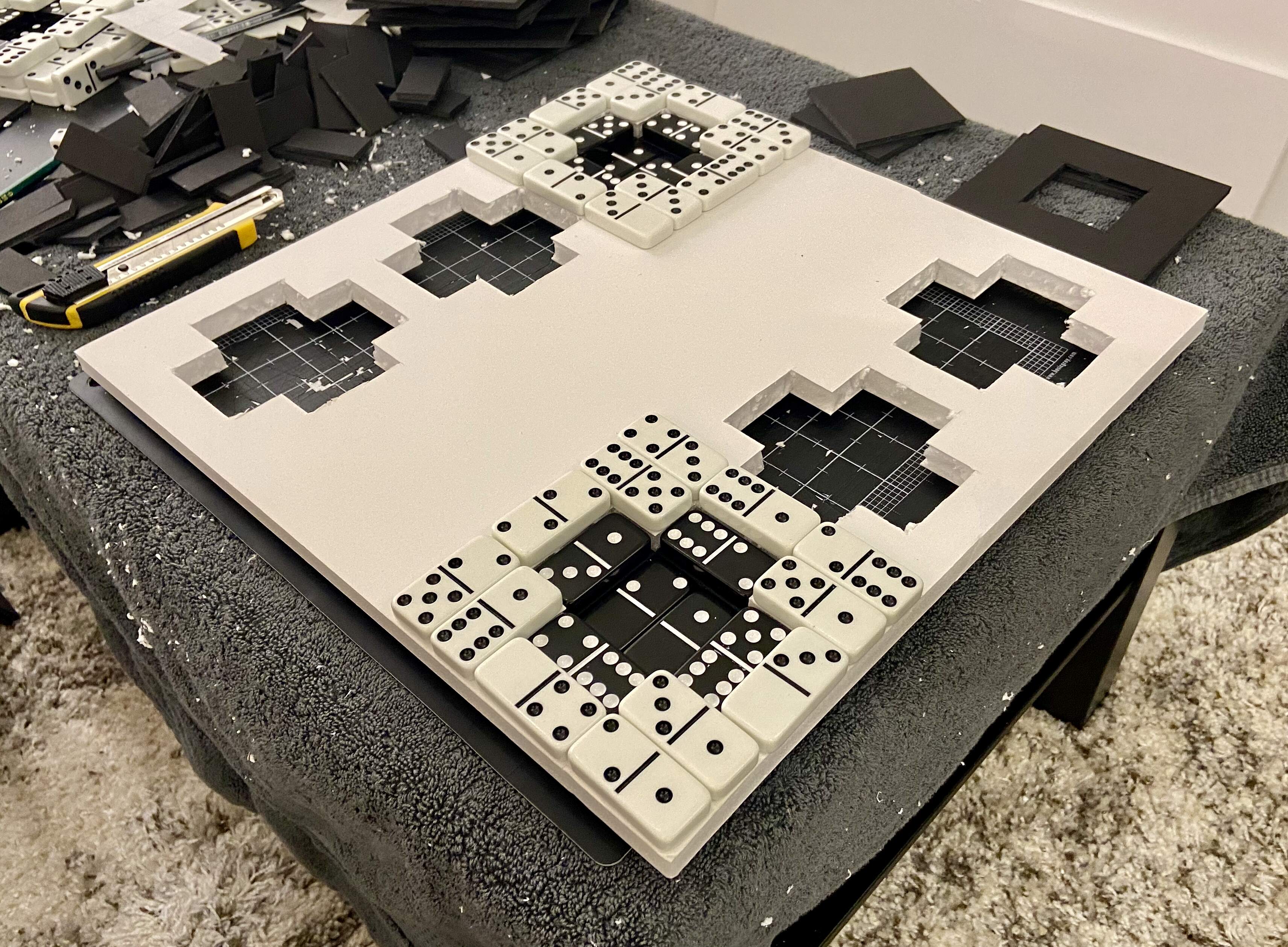
After countless hours of cutting foam board, I ended up with a die with all of its dots:
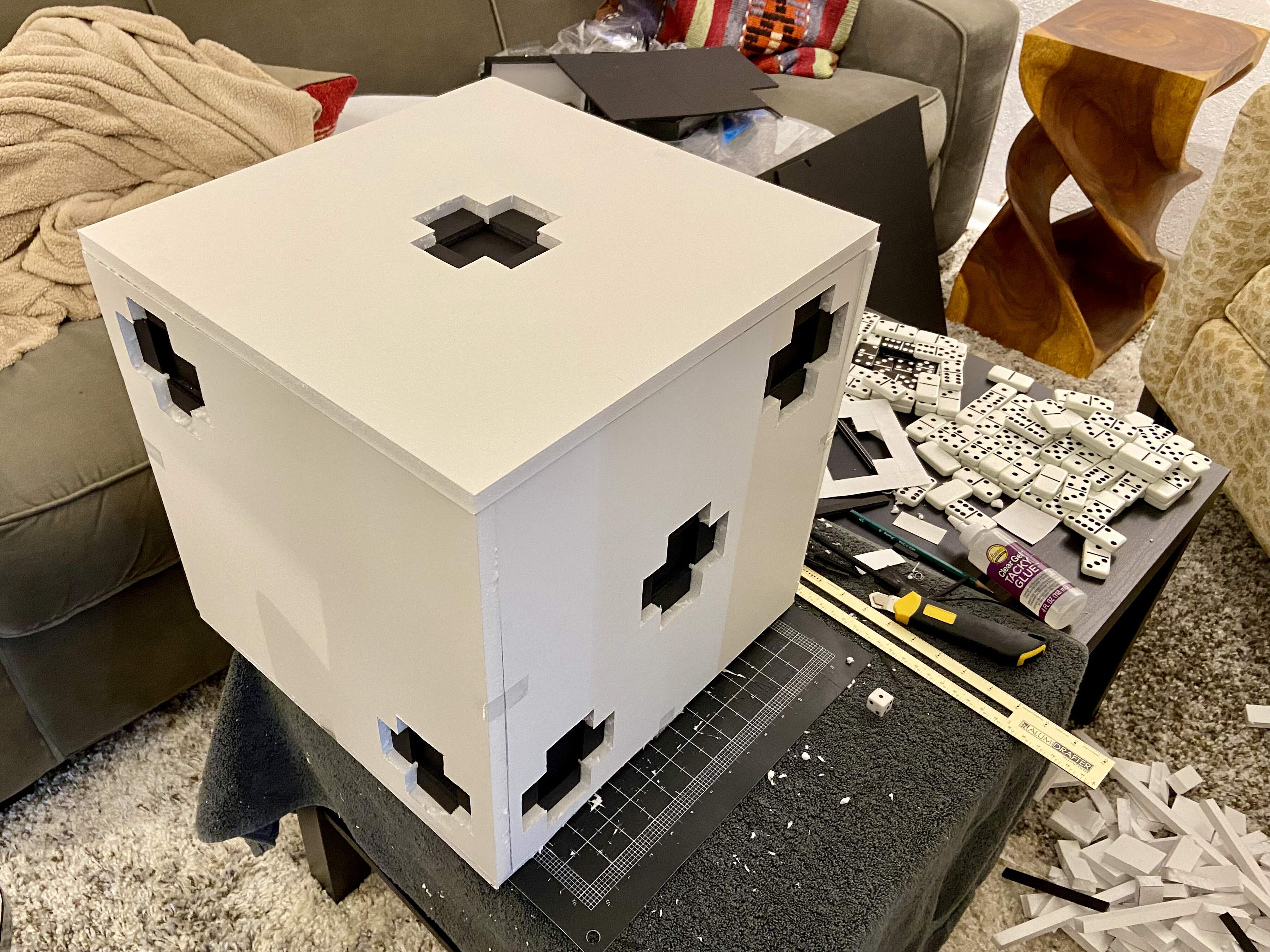
Foam board cube with dots
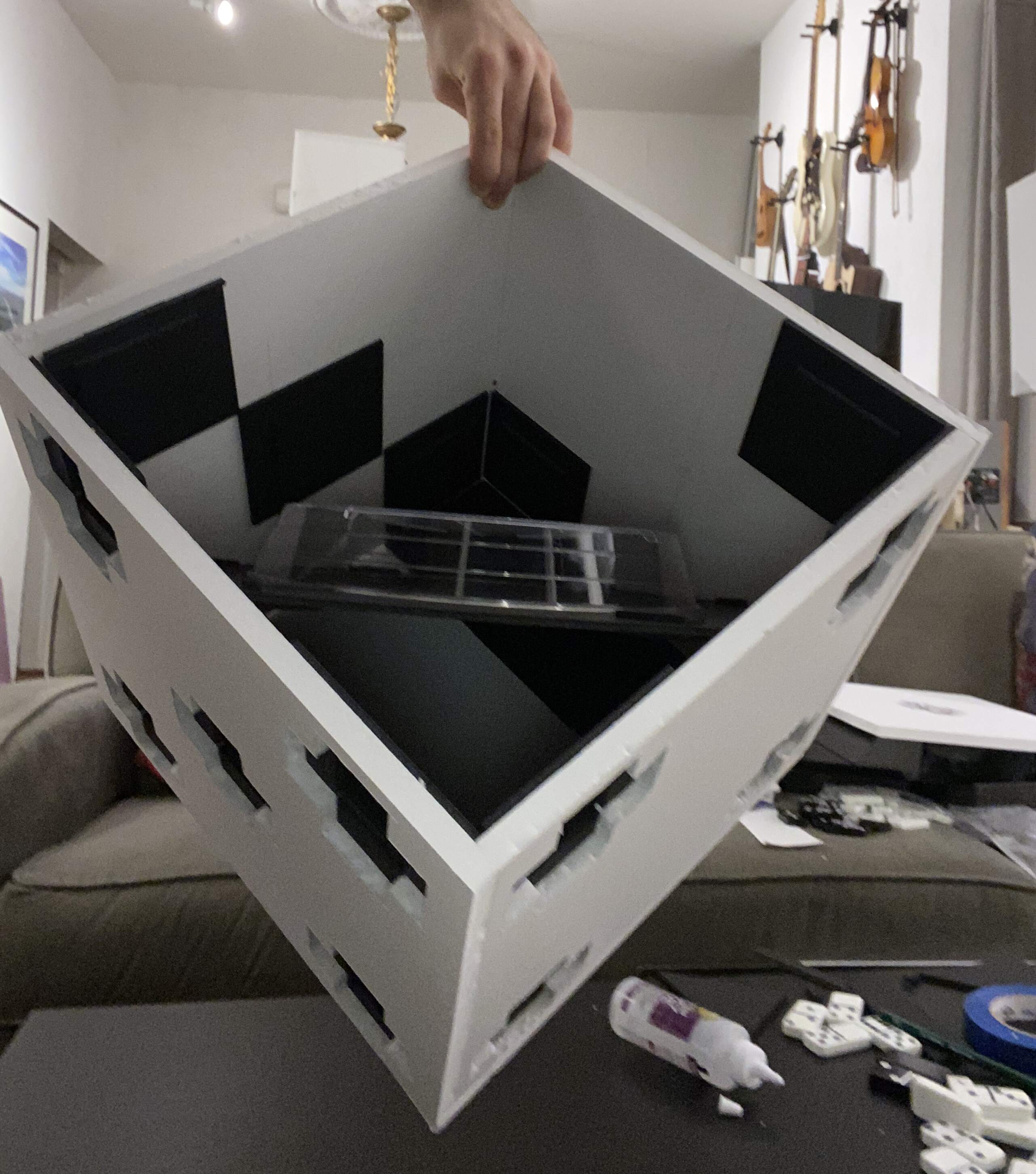
Here is the inside of the cube, before I filled it with structural supports and foam:
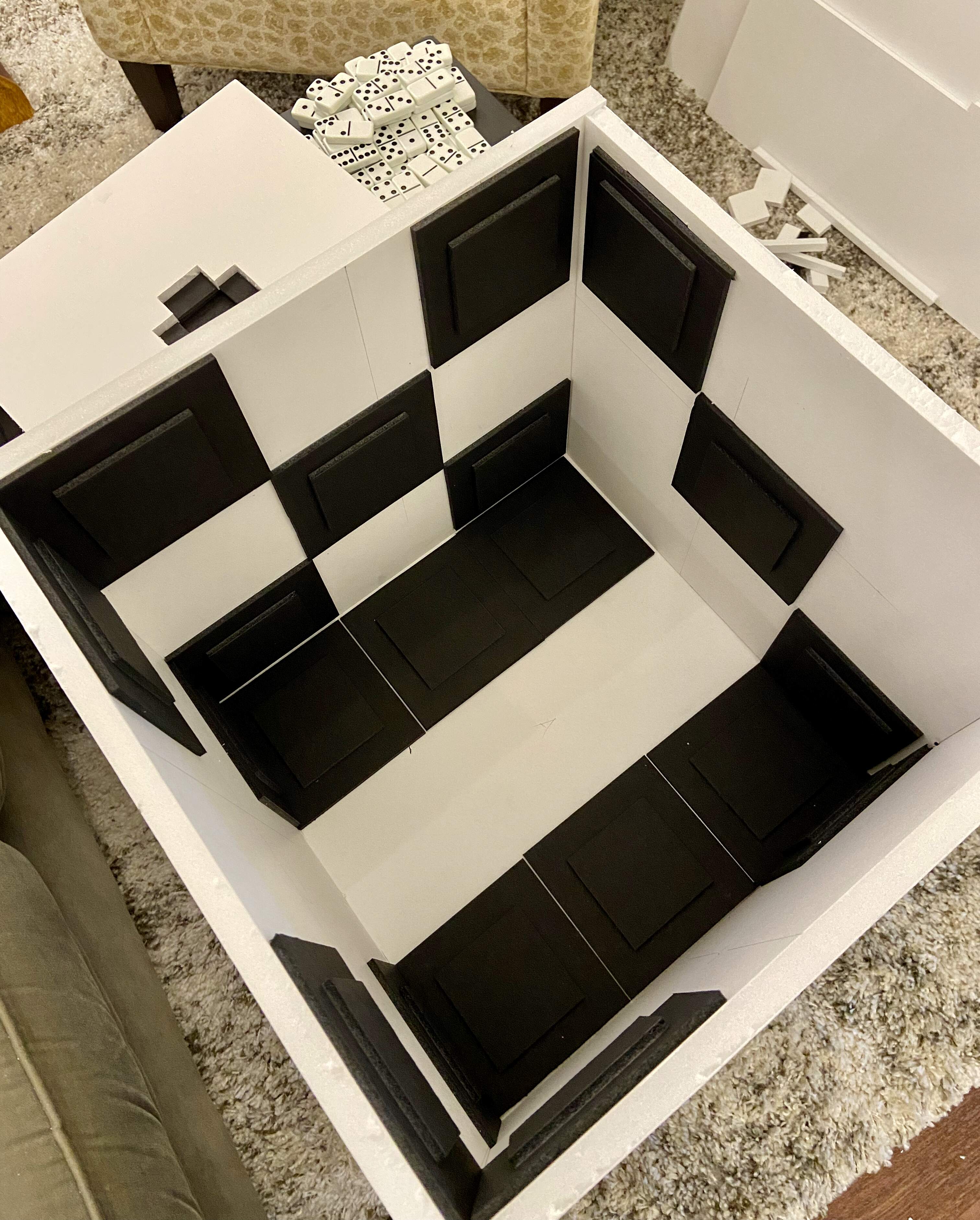
Inside the cube
To allow the die to stand on a corner, I build a support system to go inside the cube. This included a regular hexagon, based on calculations I'd done before. (Yes, the hexagon of my extremely excited notes above!)
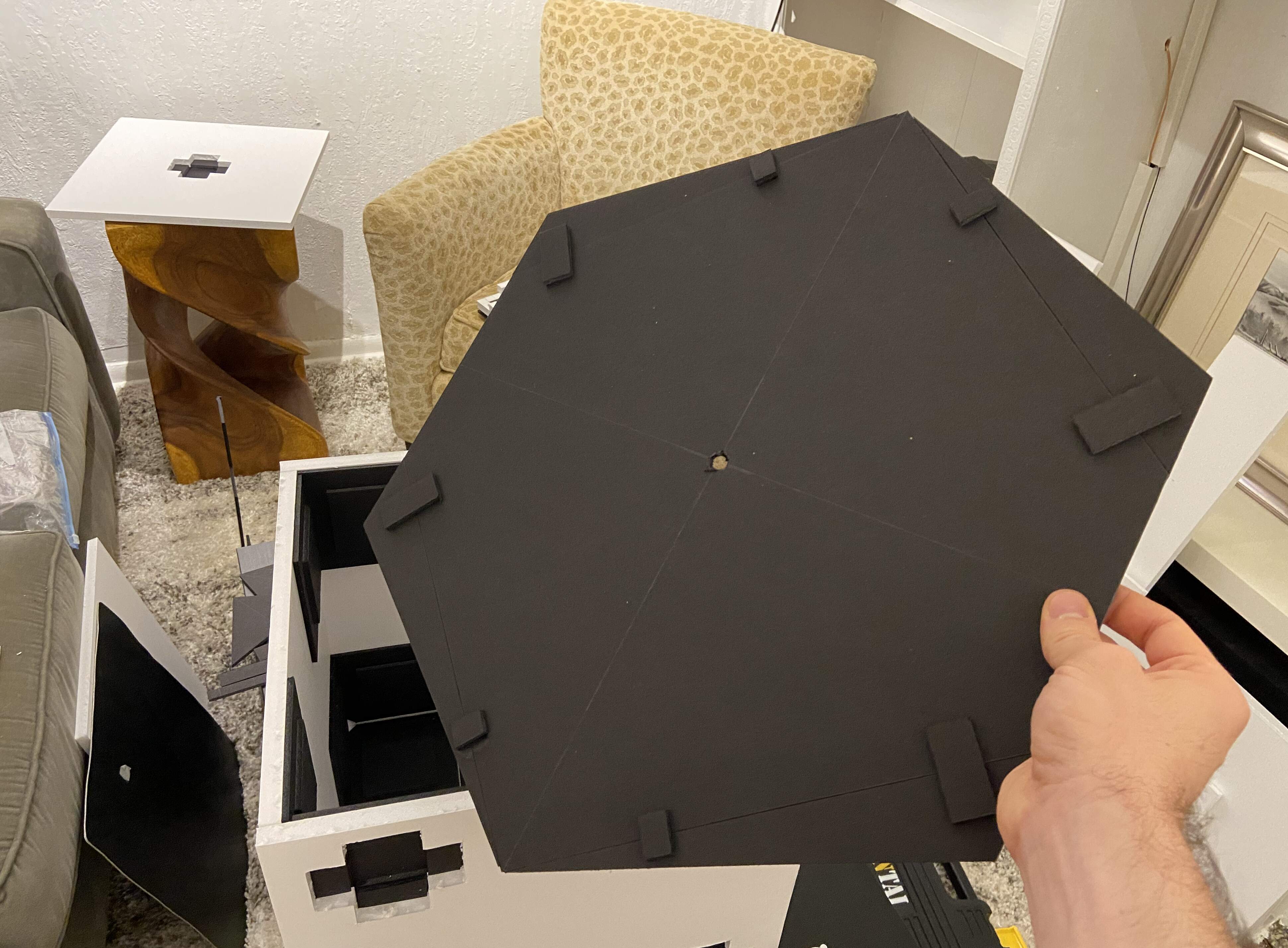
Hexagonal insert for support
This was the first time I could visually verify that my calculations had been correct, and the support system would indeed allow me to mount the die on a corner:
Cube oriented on point
Showing how internal support will work
After completing the internal support system, I filled the cube with foam, which was a total disaster! I filled the cube to the brim late at night, thinking the foam had stopped expanding, only to wake up to find that the foam had expanded way more and burst open the cube on several sides. This was the only time while making Metaphysics that I thought I might have to start over...
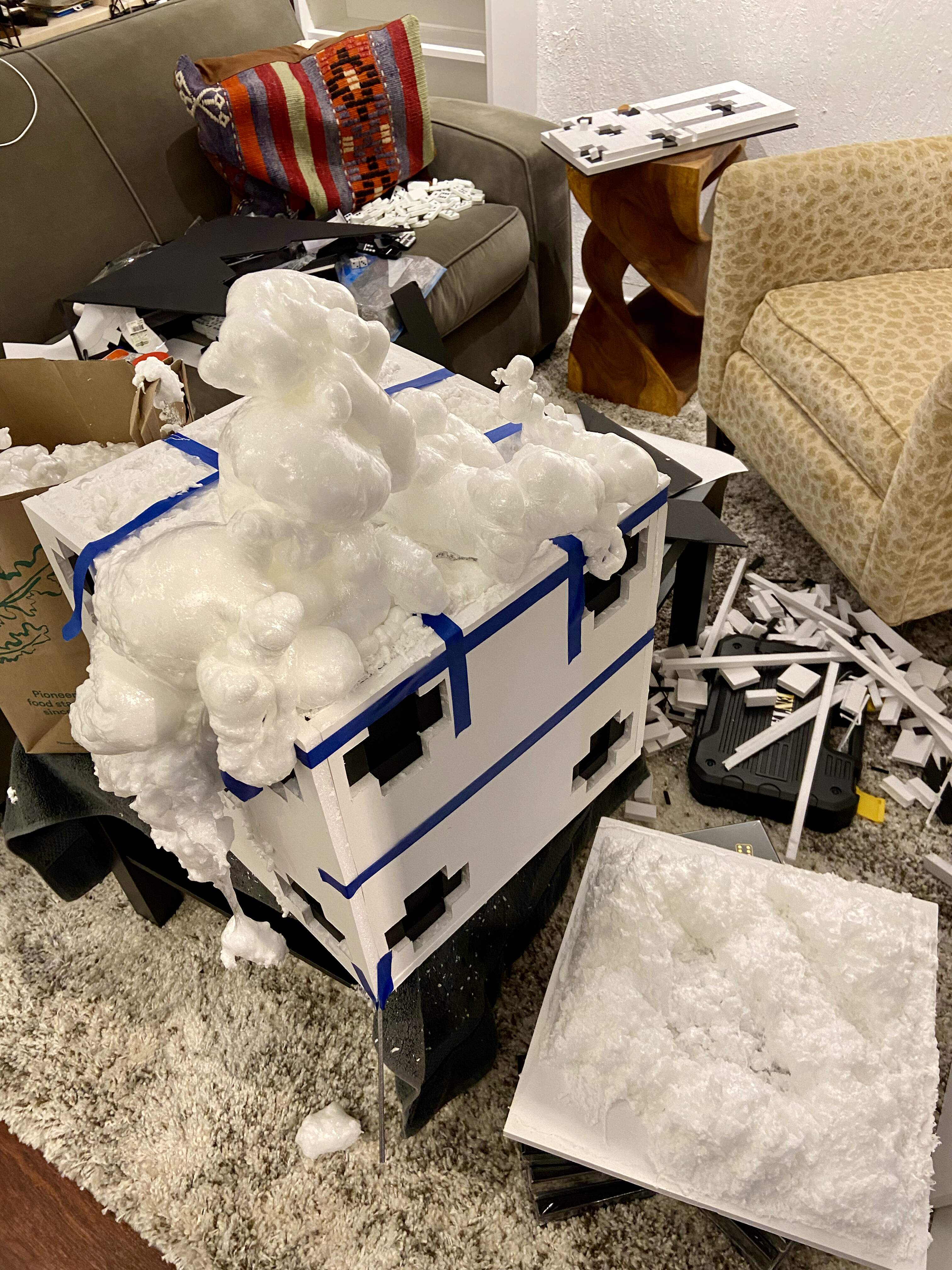
A foam disaster!
It expanded far more than anticipated
But fortunately, I was able to slice off the excess foam and salvage the cube:
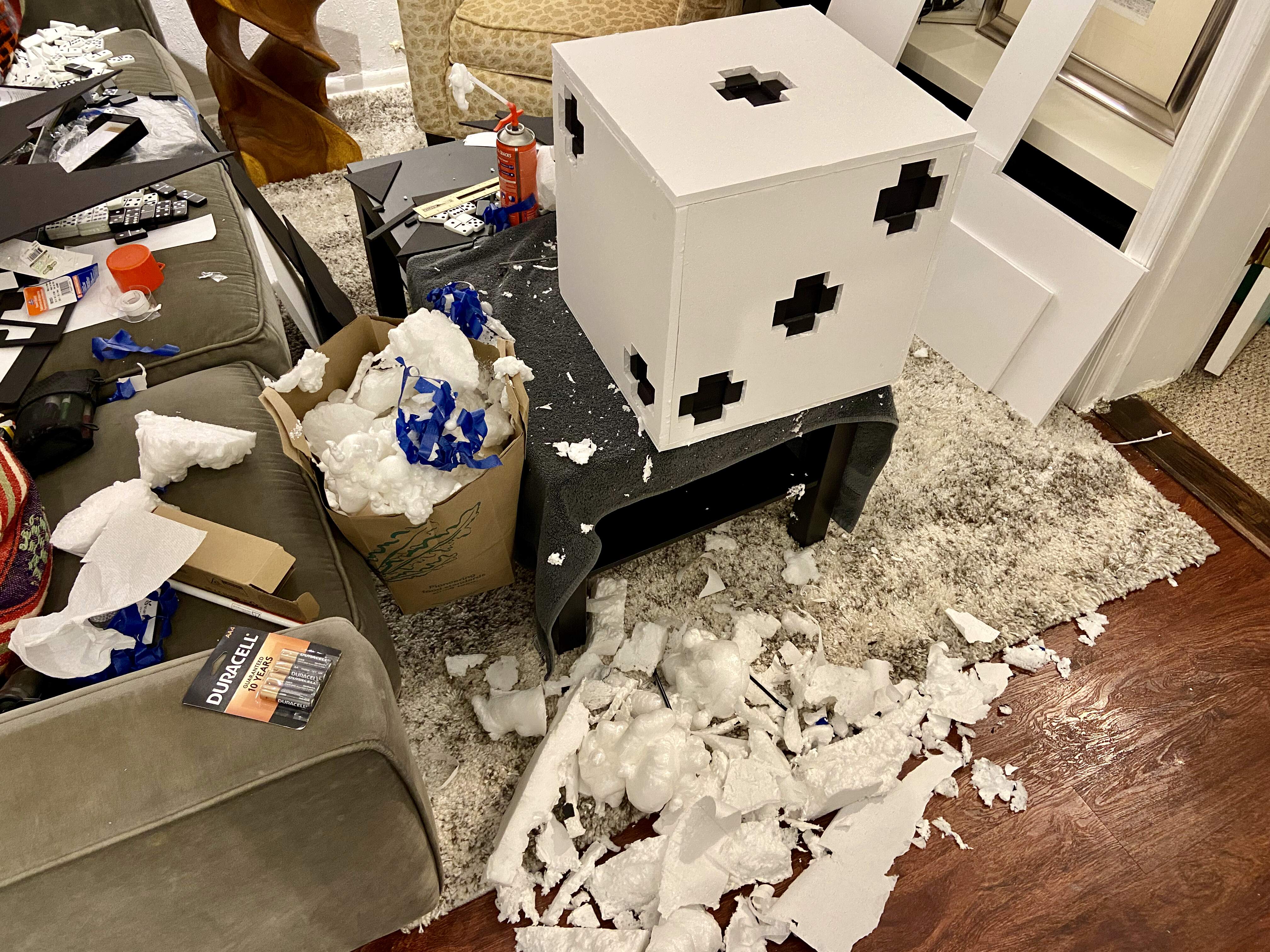
Bits of foam sliced off
Finishing side one was indescribably exciting!
Side one done
I tried to stay very organized with the dominoes, so I could easily find one of a given type. Here are the stacks I used while gluing them onto the surface of the die:
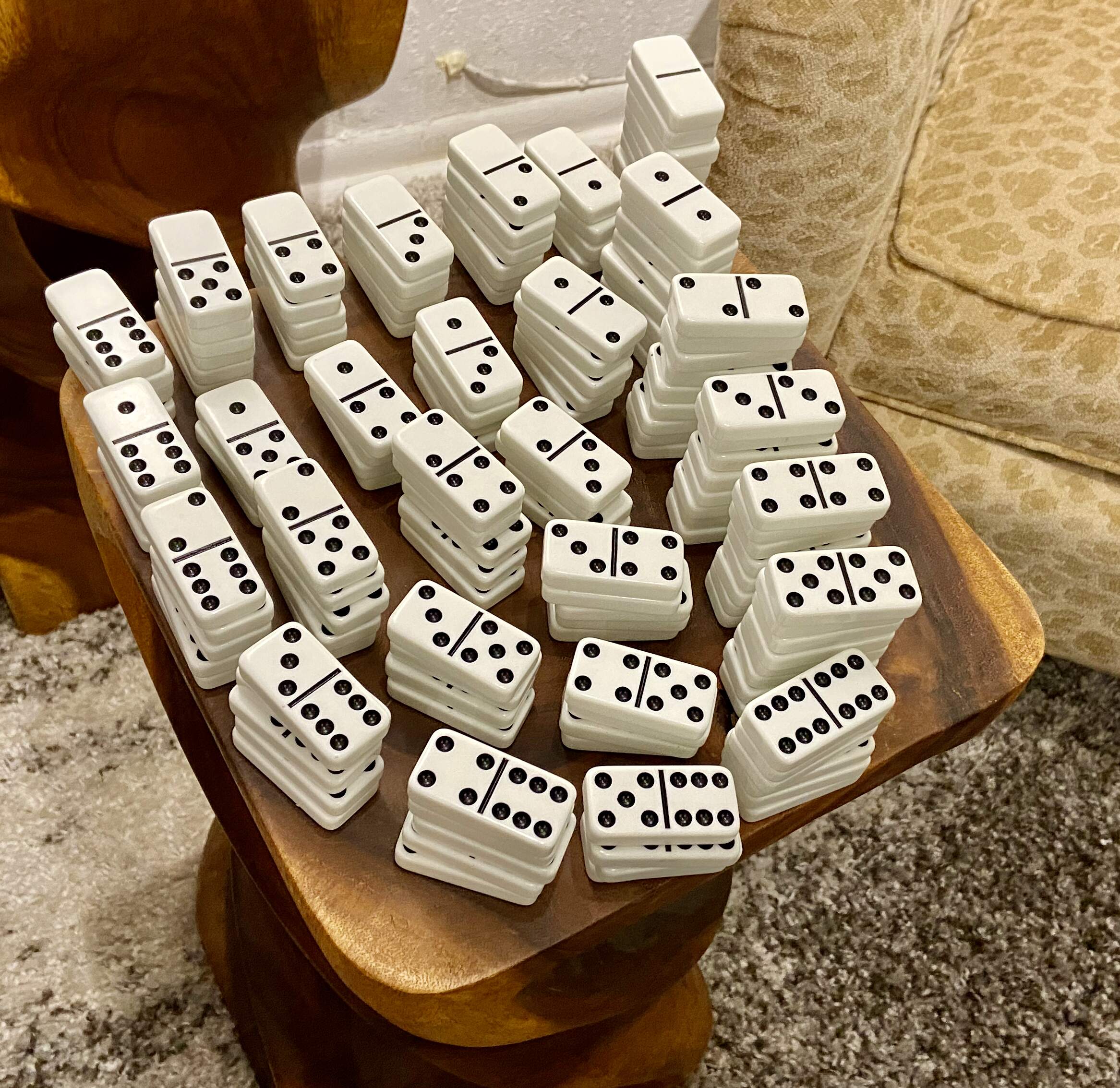
Stacks of dominoes
Each stack is of a different type
Gluing the dominoes on correctly was extremely tedious, because it required me to manually follow a specific Hilbert curve pattern and use the values of my Wallis-like domino train product. This is one example of where my code was especially helpful because it allowed me to create an exact, color coded sequence of dominoes:
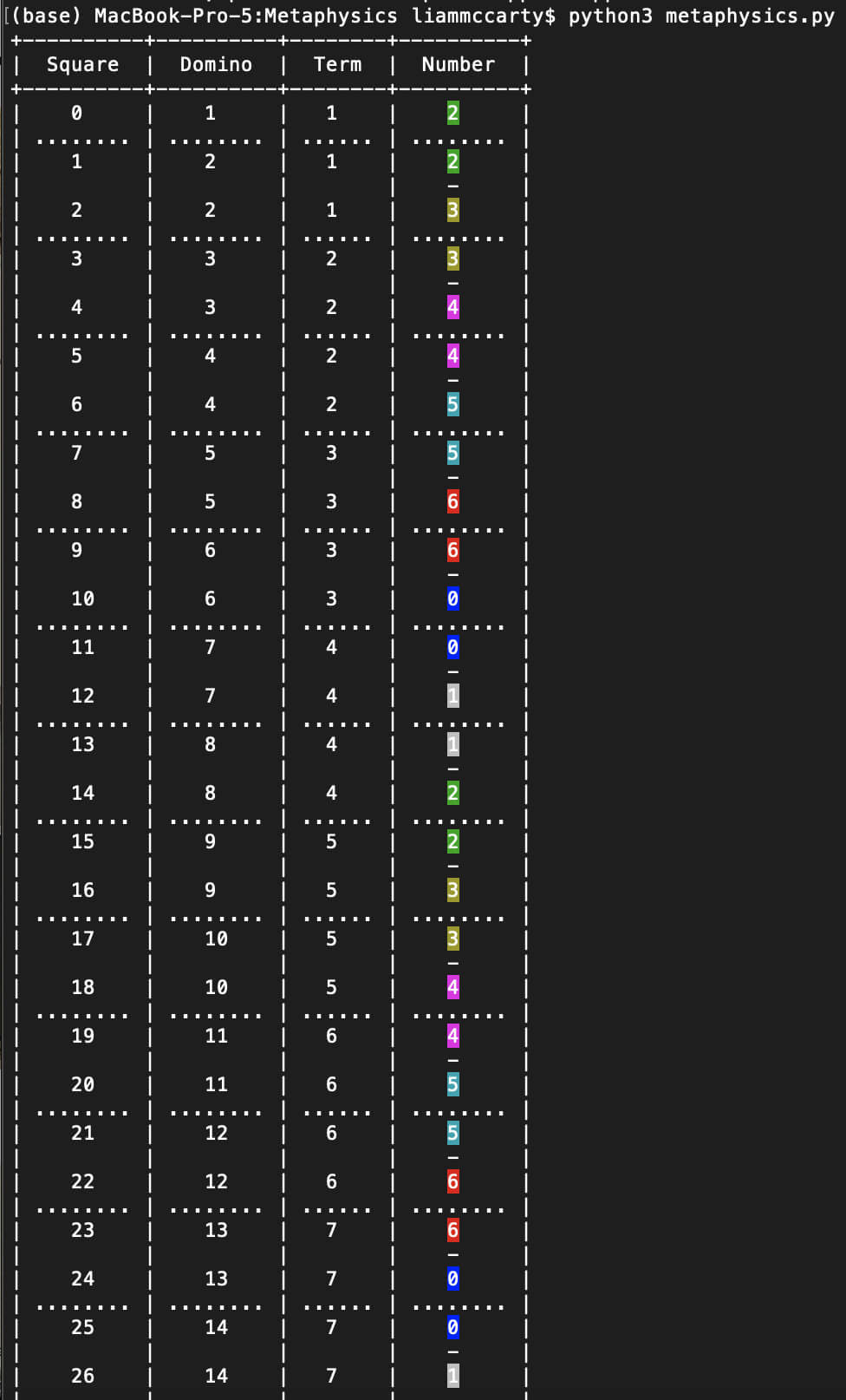
Terminal output (fragment) of my code
See print_values() for details
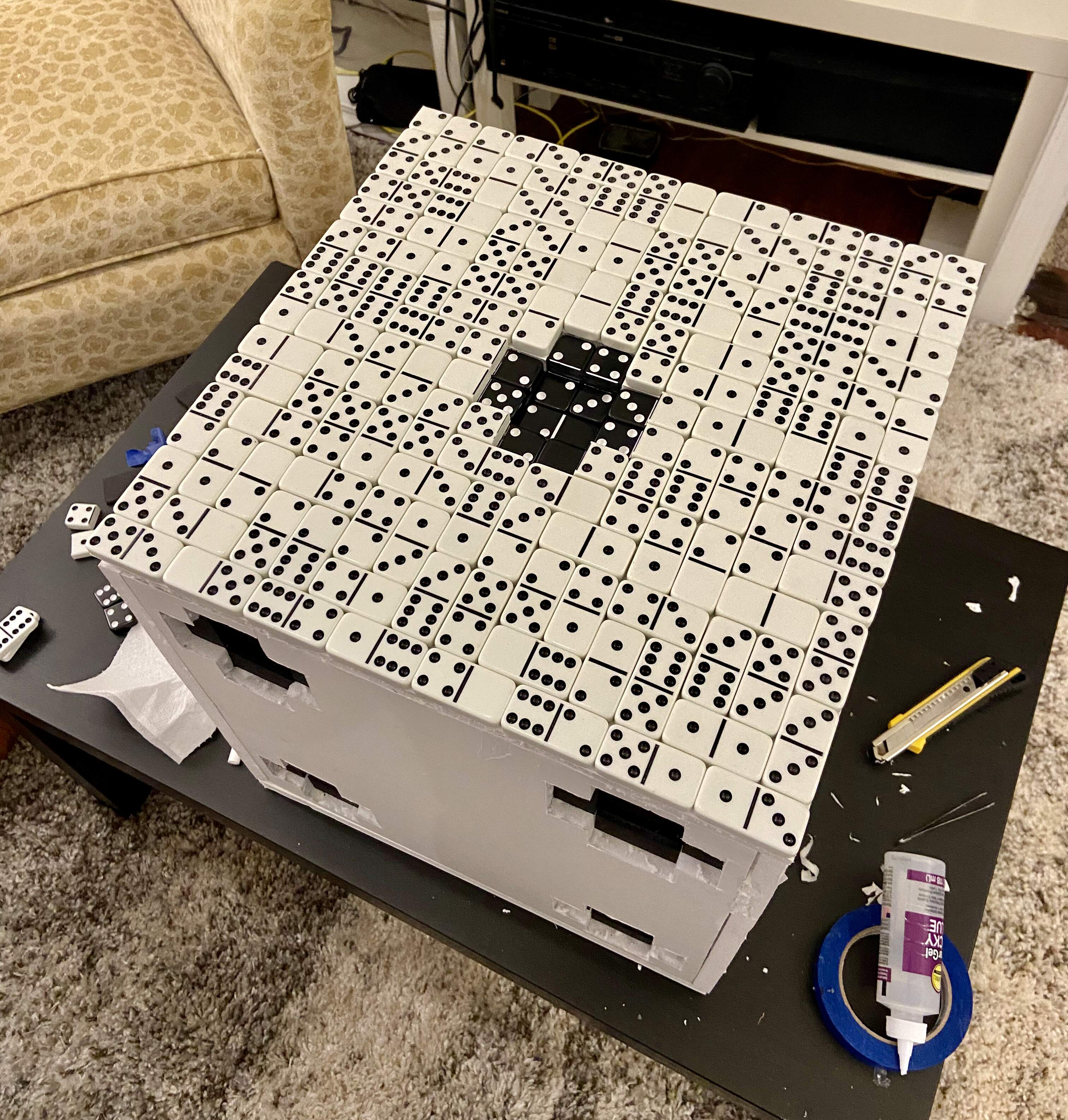
Here is side two, in the middle of the tiling process:
Part of side two done
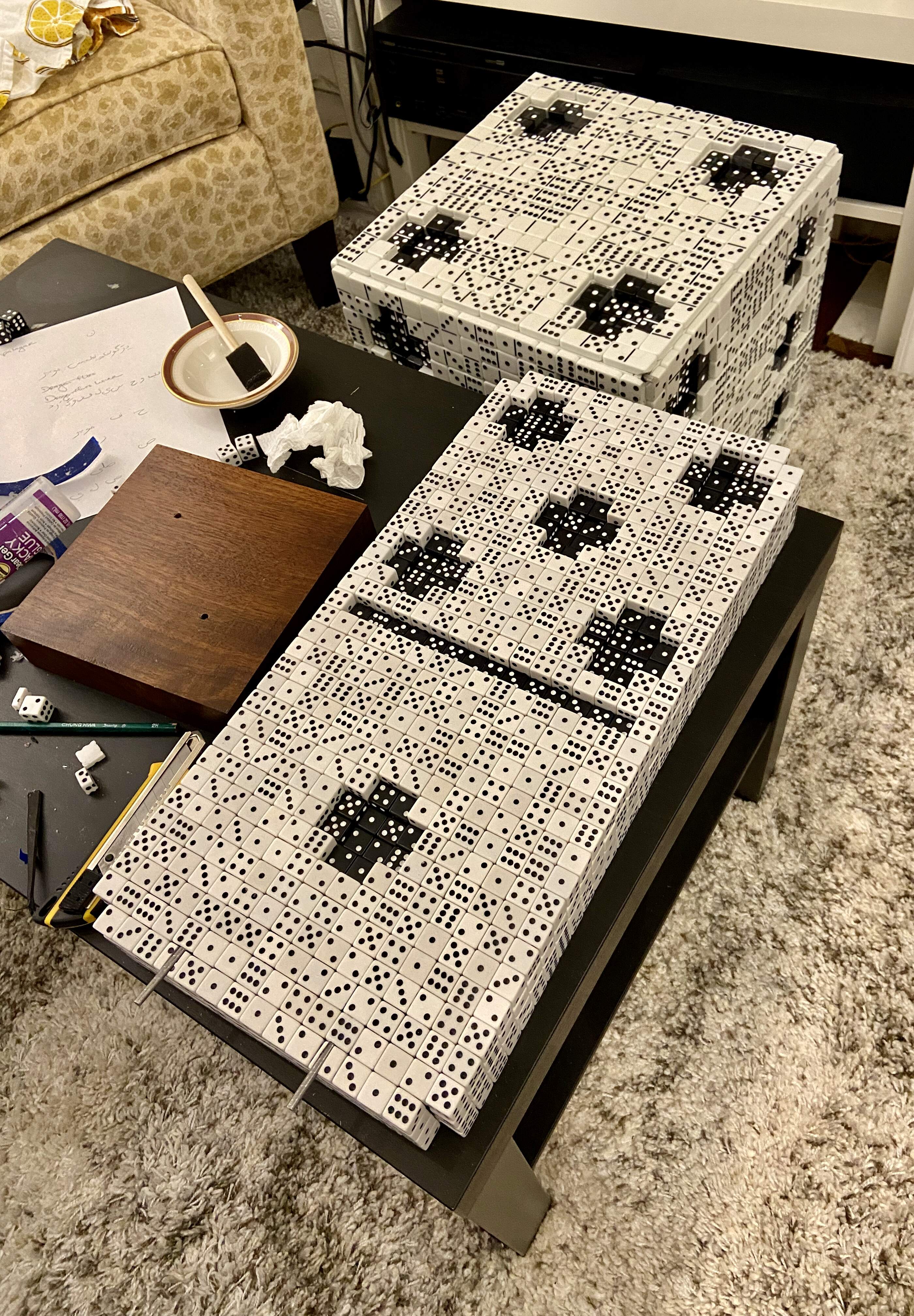
With three sides done, the die was starting to look fantastic:
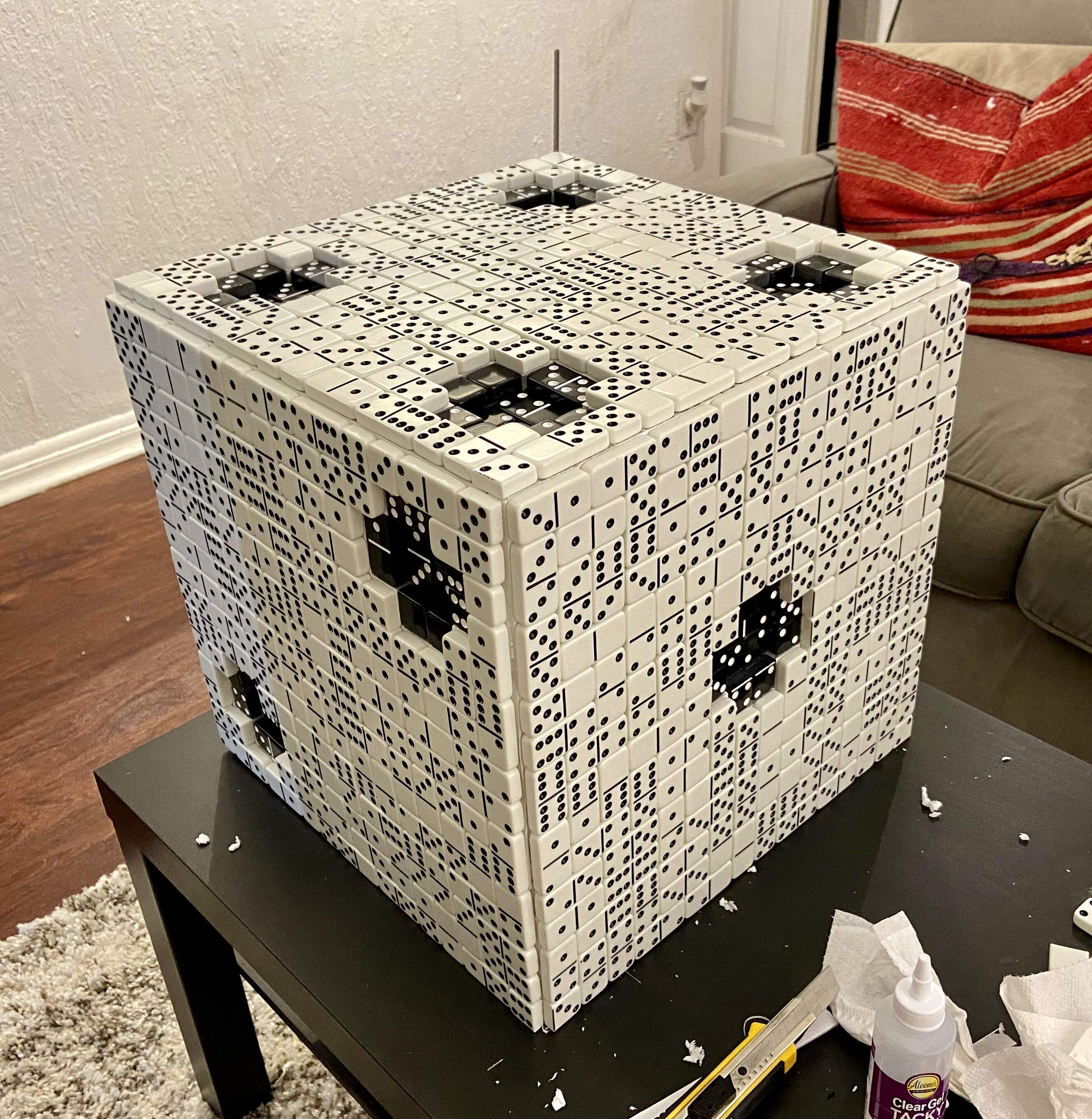
Three sides done
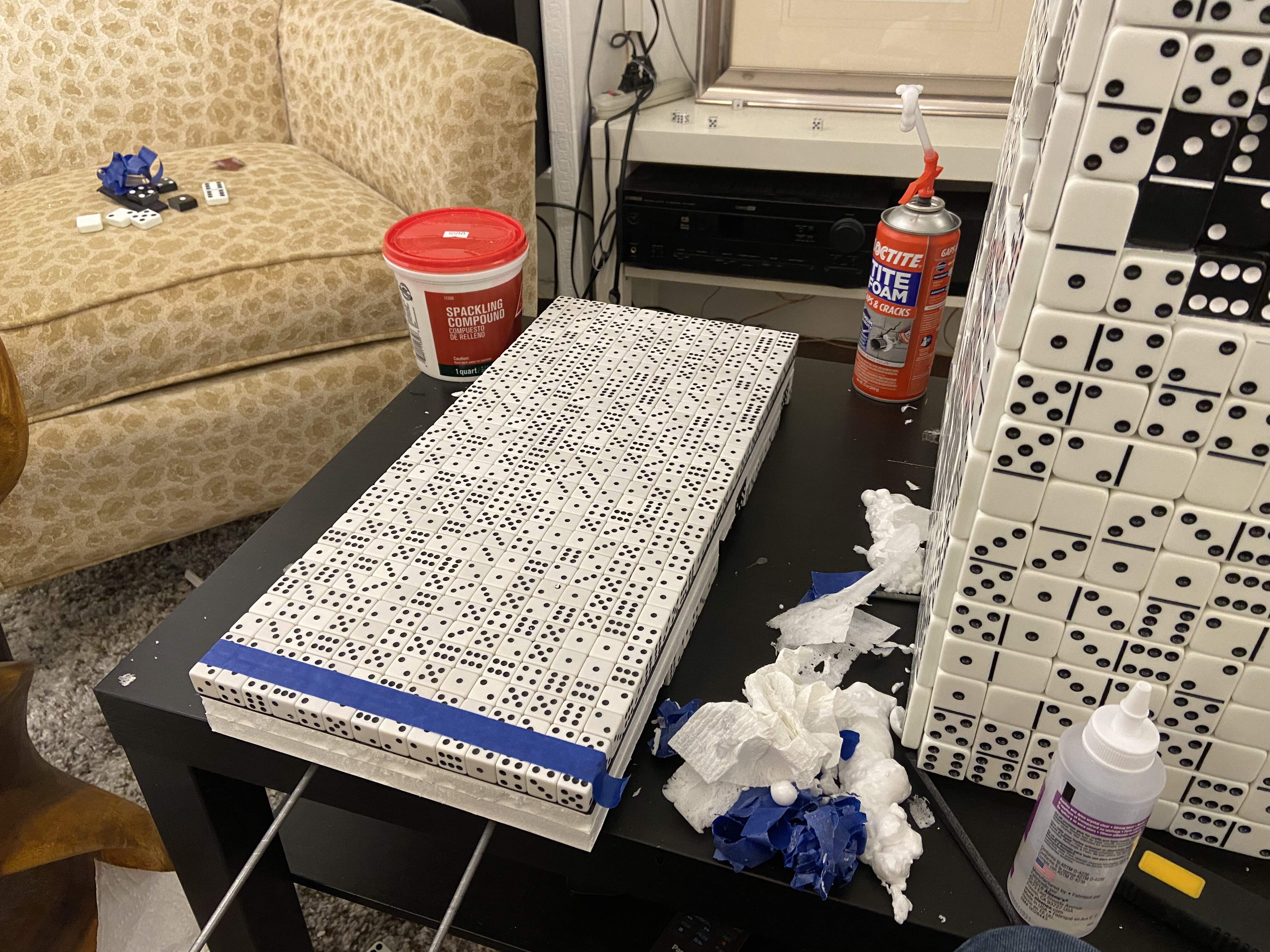
I used all sorts of random things to weight down the domino of dice as the glue between the foam board pieces dried, so it wouldn't warp:
Holding the domino of dice down
Ensuring it wouldn't warp as the glue dried
Before gluing on all of the dice, I made sure I had cut the foam board correctly to make the dots. It looked great!
Testing the dots on the domino
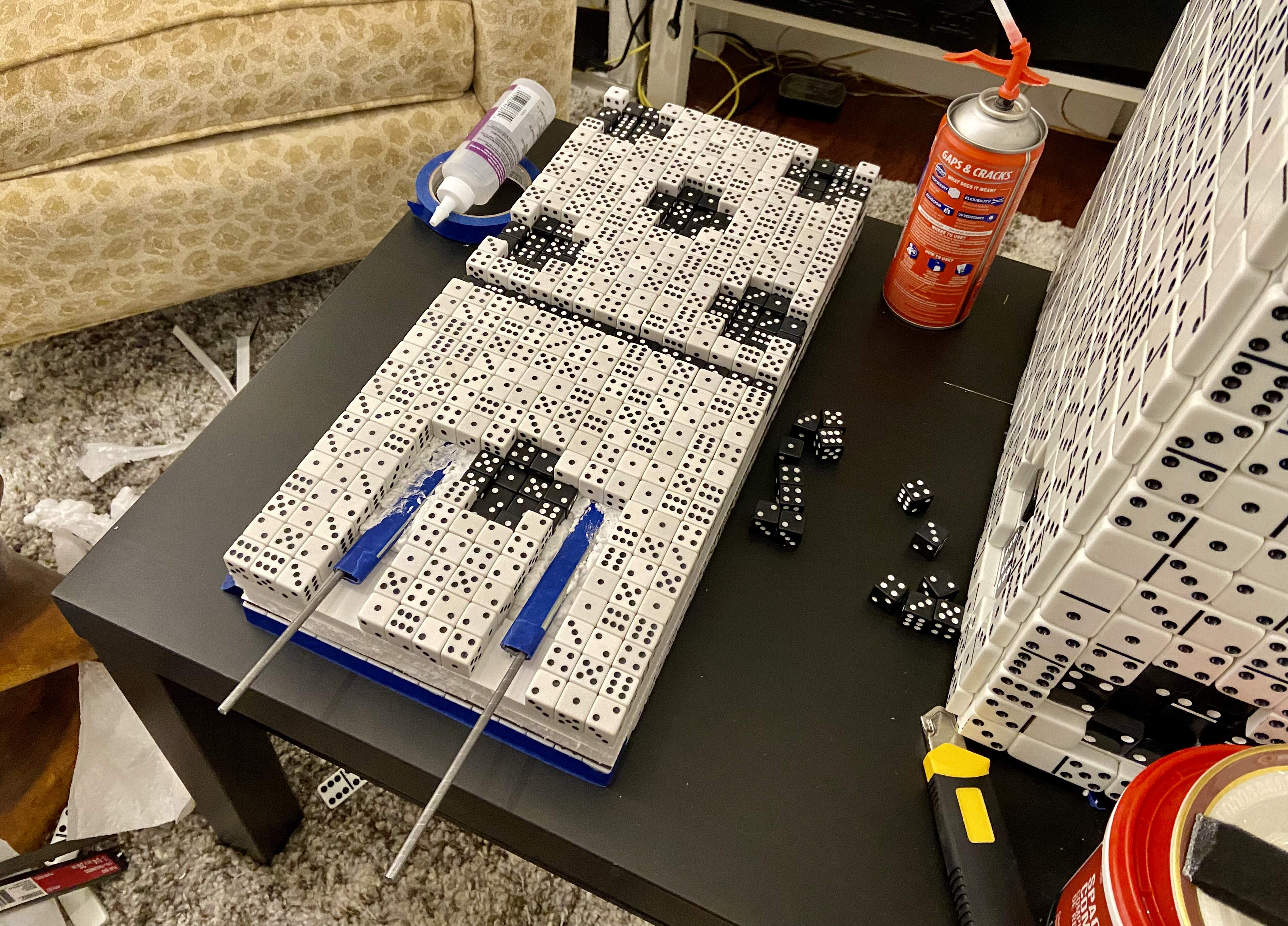
I settled on using these rails as a support system for metal rods that would prop up the domino:
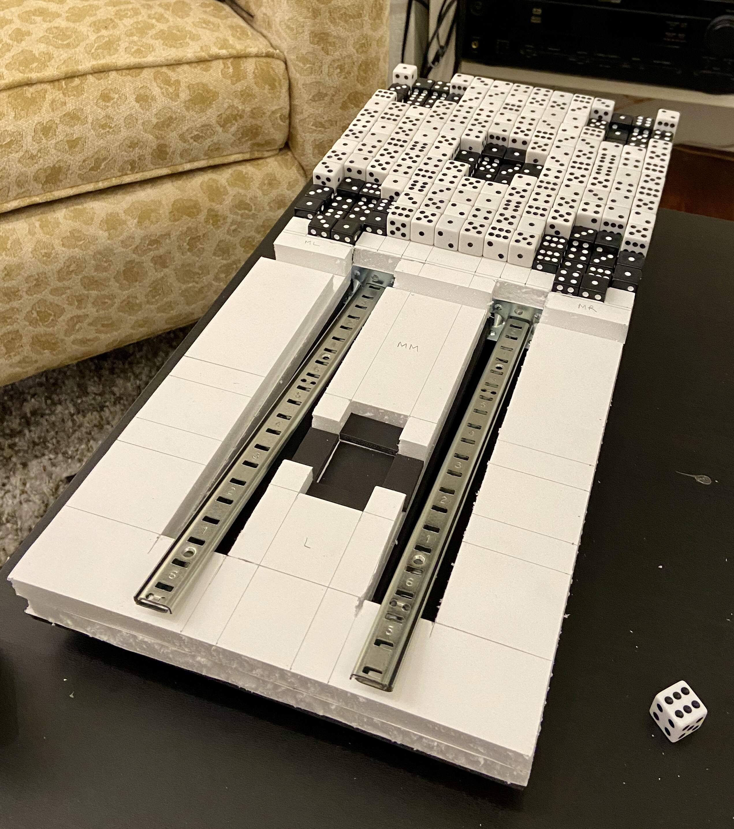
Support rails for the domino
I had to work very hard to make sure the structural system for the domino wouldn't move around as the foam I would add expanded. I had learned my lesson from the die of dominoes foam disaster!
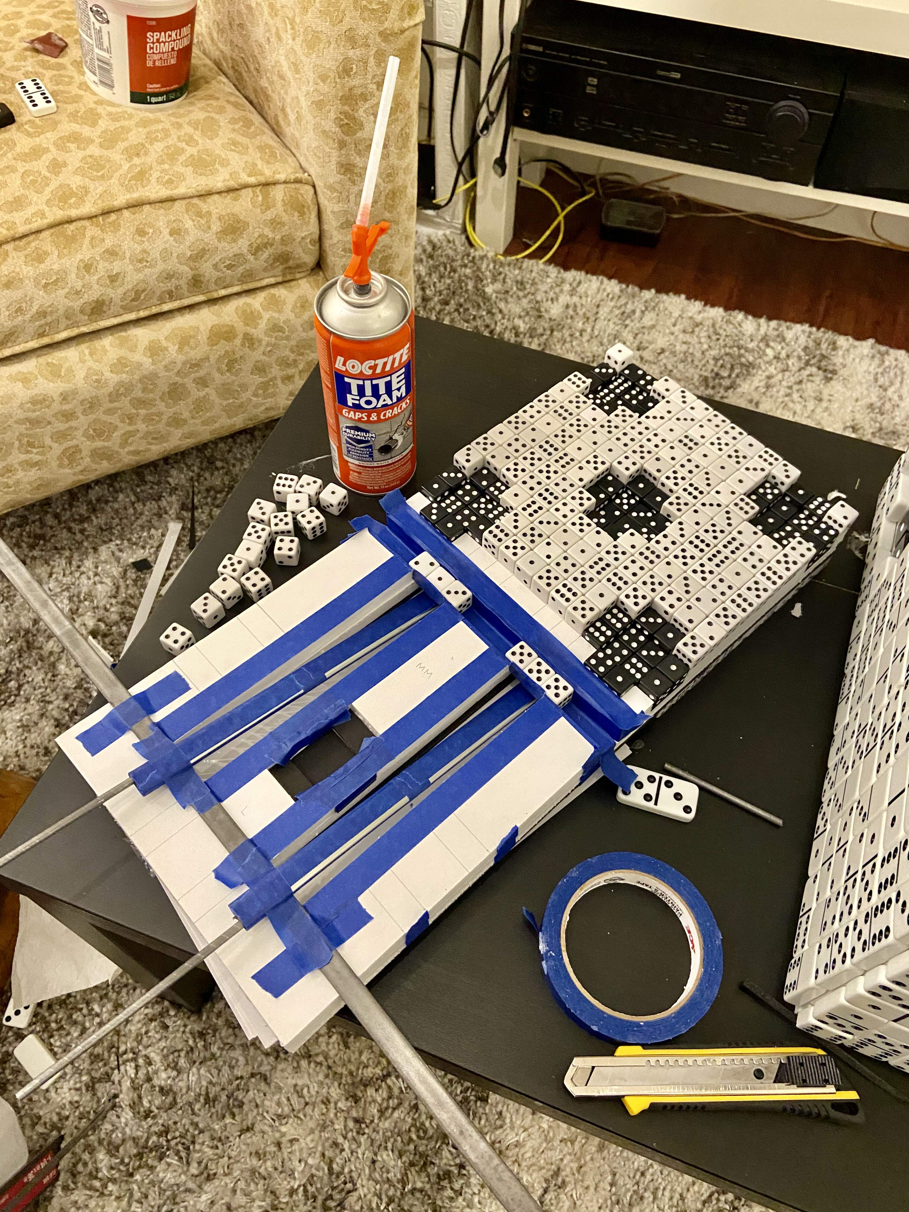
Carefully holding parts of the domino in place
Ensuring the foam I would add wouldn't move things as it expanded
Here is the back of the domino of dice, partly done:
Part of the domino back done
And here it is fully done:
All of the domino back done
I painstakingly painted thin lines of glow in the dark paint on the surface of the die of dominoes. I had to be especially careful to ensure the lines stayed as straight as possible and just the right thickness to be unnoticeable with the lights on but bright with the lights off.
Painting lines of glow in the dark paint
After countless hours of tweaking, I finally embedded the full support system for the domino of dice:
The domino with supports
When I finished painting the first side (I started with side six) and turned the lights off... I was stunned! The pattern was ghostly and beautiful.
Side six glowing in the dark!
My iPhone automatically brightened this image. It was pitch black in the room apart from the glowing paint.
At long last, I attached the base to the domino...
The domino with its base
... and stood it up! This was utterly terrifying, and then utterly thrilling.
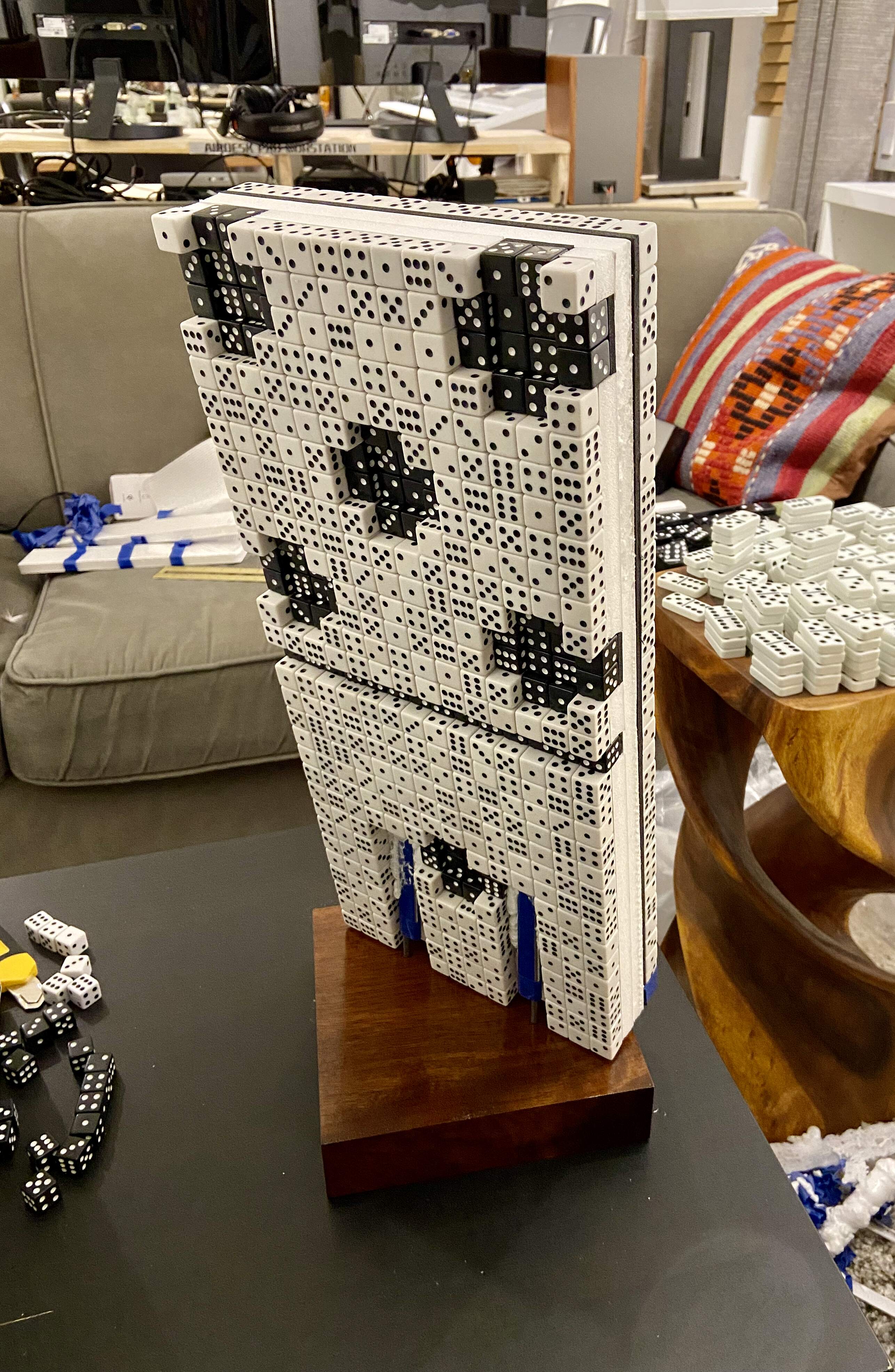
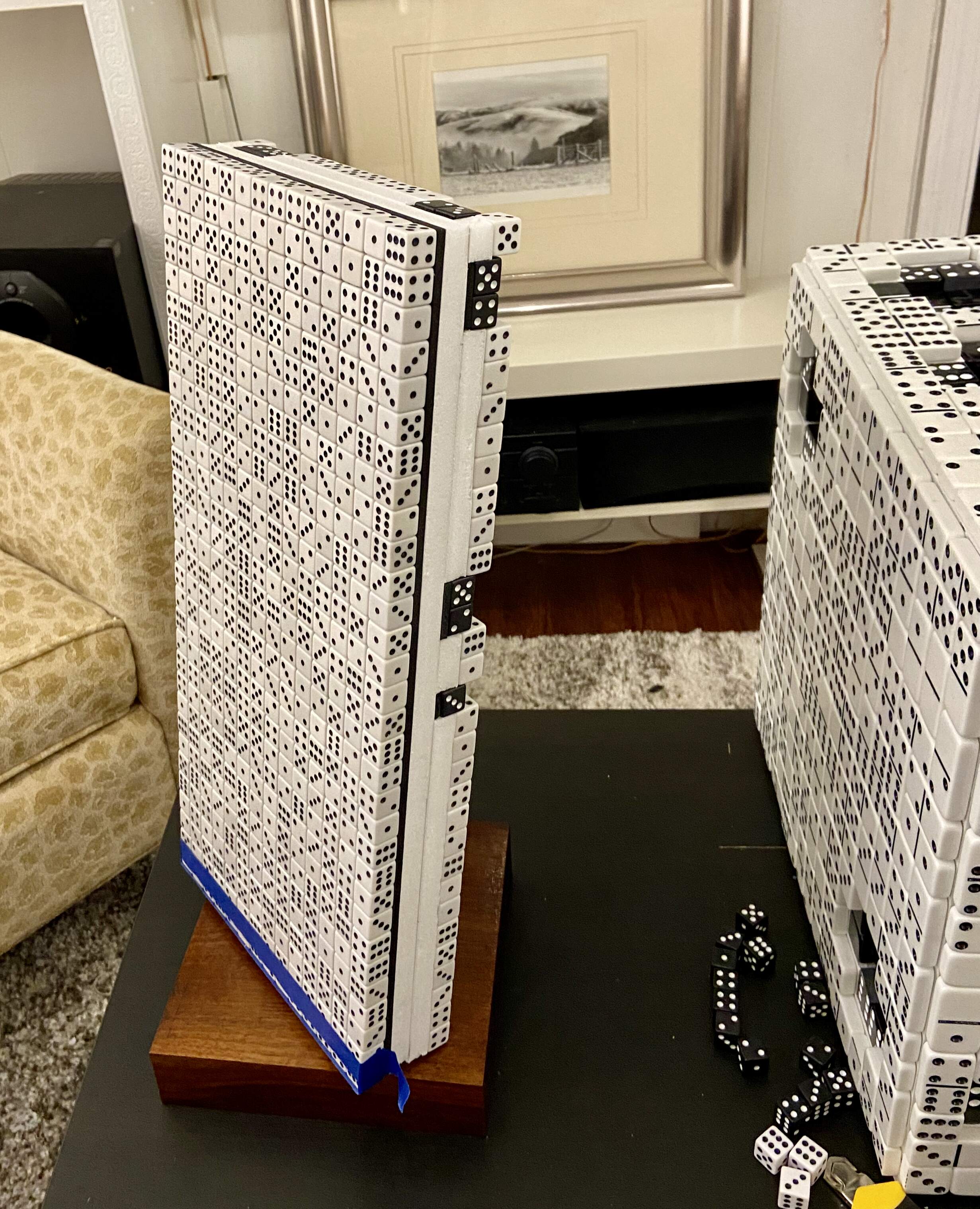
The domino finally standing up!
(front)
Here it is from the back:
The domino finally standing up!
(back))
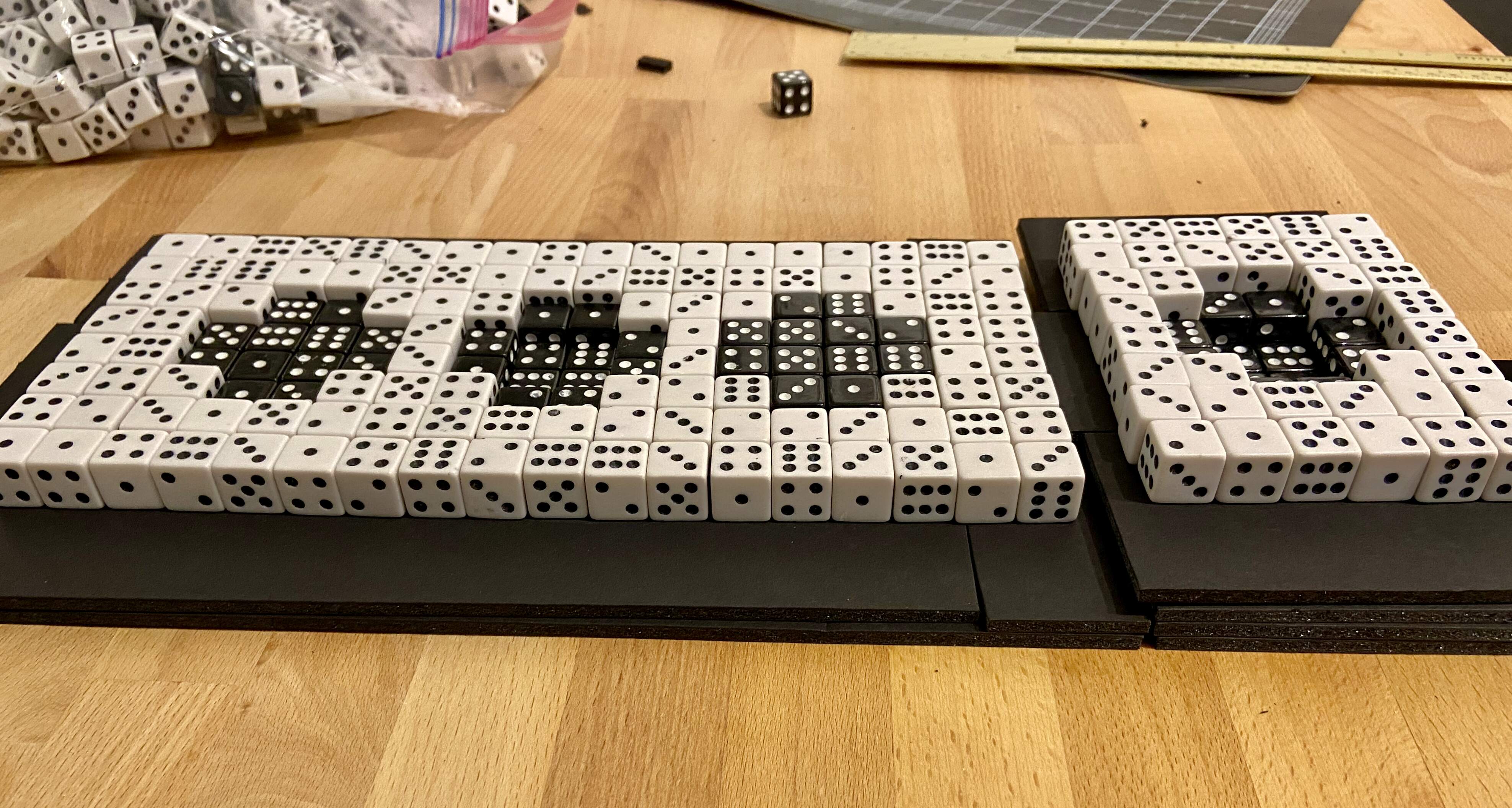
Covering up the support system with dice was extraordinarily difficult because I had to slice each die at very specific angles so it would rest on top of the supports while staying flush with the other dice. But, eventually, I got it to work:
The domino almost done
Lastly, triumphantly, I signed the backs of the sculpture bases and finished Metaphysics!
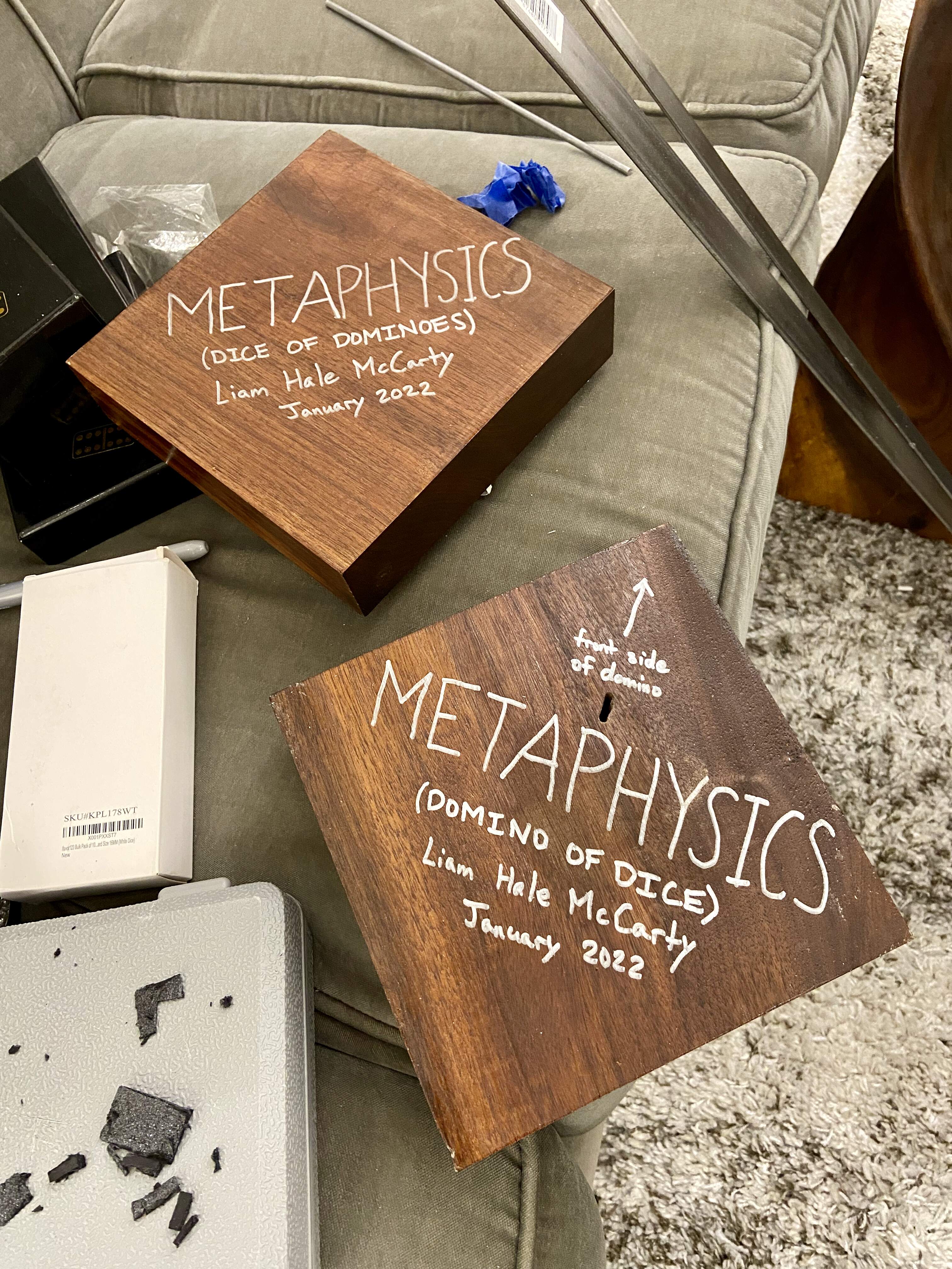
Backs of the sculpture bases
Math
This section provides a deep dive into the math behind Metaphysics.
For the die of dominoes, I wanted the tiling of dominoes to represent (or a multiple of it), which captures the duality between determinism and randomness the piece is about. Because the tiling follows a Hilbert curve pattern, it needs to be a domino train: a series of dominoes that have matching numbers end to end. Further, it needs to be a circular domino train — one that loops back on itself — since the tiling covers a closed surface. To satisfy these constraints, I needed a very particular formulation.
Domino-ifying the Wallis Product
The Wallis product is a famous formula for :
If this doesn't amaze you, stop for a moment to think about it. Somehow, by multiplying pairs of fractions — one a bit larger and the other a bit smaller than — infinitely many times, we end up with exactly . Wow!
This product has some nice properties. For one, its terms are fractions, and dominoes themselves look like fractions in that they have two numbers separated by a line. For another, the two fractions in each term share a number, and so do the neighboring fractions in adjacent terms, so all of the fractions can be "aligned" domino train style.
Modulo 7
There are just a few issues. One is that the numbers in the Wallis product grow infinitely large, while domino numbers are never greater than 6. There's a simple fix for this. I'll just write the numbers to create a Wallis-like product:
There are two related concepts that are helpful to know here: base and modulo.
Base just refers the number of digits used to represent numbers. Most numbers in everyday life are written base 10, since they use 10 digits: 0 through 9. But dominoes are base 7, since they use only 7 digits: 0 through 6.
Modulo, or just "mod", basically just means "remainder". It's easiest to see how this works with an example (using standard base 10). because . An everyday example is that people usually tell time . For example, 3:00 PM is just 15:00 !
If your alarm bells are going off – eek, he's dividing by zero! – remember that the goal is to "domino-ify" the Wallis product so it's suitable for a domino train. Dominoes "divide by zero" in the sense that the "fractions" they represent can have zero in either the numerator or denominator, so it's not a problem to divide by zero here.
All of the numbers, including zero, are really just labels. I could replace them with emojis, made up symbols, names of sports teams, or anything else, and there wouldn't be any issue.
Cycling
Another small issue is that this Wallis-like product repeats so quickly (after just seven terms) that it doesn't cycle through all possible dominoes. The repeating unit is:
So, for example, no double like ever appears. This means I would need a huge number of domino sets, since I wouldn't be using very many dominoes from each set.
This also makes the Wallis-like product less in keeping with the original Wallis product, since it retains no hint of the infinite increase in the numbers. Because retains only the remainder, any record of the quotient is lost.
Again, there's a simple fix. Every time the unit above repeats, we'll just add 1 to the numerators of the fractions:
This is isn't as complicated as it looks. starts at 0 when and hits 1 when , 2 when , and so on. In between those values of , it's a non-integer value. For example, when it's . So to make sure it's always an integer, we'll just "lop off" the decimal part using , the floor function of .
The formula above uses the "floor function", which cuts off any non-integer parts of a number (the part after the decimal point). For example, the floor function of 6.2 is 6, and the floor function of 101.89712 is 101. The name is intuitive if you think of each "floor" as an integer (0, 1, 2, 3, ...). If a number is "between the floors", the floor function takes it back down to the floor.
Fun fact: there's also a "ceiling function", which does what it sounds like!
Then, the first unit is as above, the second is
the third is
and so on. Note that now the repeating unit is 49 terms — 7 times as long as the original one because it takes seven iterations of the unit to "loop back" to the first one.
Flipping Fractions
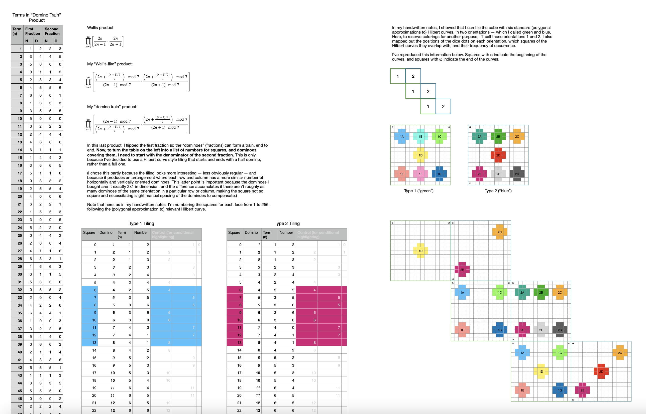
There's just one more change to make. To make a domino train, I need the denominator of the first fraction in a term to match the numerator of the second fraction in that same term, and I need the denominator of the second fraction in a term to match the numerator of the first fraction in the next term. To accomplish this, I only need to flip the first fraction in each term, which results in my final Wallis-like domino train product:
Now, the first unit is
the second is
and so on.
Boundary Conditions
One detail that's worth noting concerns boundary conditions. For Metaphysics, the global Hilbert curve is closed, so the domino train needs to "loop back on itself". This is a boundary condition that requires the total number of dominoes to be a multiple of the number of dominoes in a repeating unit, which is . For (positive integer) side length , the number of dominoes per side is , so the total number of dominoes (for all 6 sides) is .
This is a difficult constraint to satisfy, especially at small scale, because there's another constraint that must be simultaneously satisfied: the side length must be a power of 2 because each side is covered by a Hilbert curve. In other words, for some (positive integer) power .
So, the two constraints are and . Therefore, or, written slightly differently, for some positive integer . And thus:
When I try to solve this equation (with WolframAlpha), the result is "no integer solutions". So, it's not just difficult to solve — it's impossible!
But, fortunately, I have a simple way around this problem. Each local Hilbert curve corresponds to not just one but two valid tiling patterns. One pattern starts and ends with a full domino, but the other starts and ends with a half domino. I prefer the latter for a few reasons:
- It's not "self contained" and implies that the tiling extends beyond a single side of the cube.
- It looks more interesting and less obviously regular than the other tiling.
- It has rows and columns with more similar numbers of horizontally and vertically oriented dominoes than the other tiling. (The other tiling, for example, has two rows with all vertically oriented dominoes.)
The last point is important because real (standard) dominoes have a length to width ratio that's almost but not exactly 2:1, and the slight difference between length and width accumulates when there aren't similar numbers of dominoes in each orientation. This makes the arrangement not quite square, requiring slight manual adjustment that's hard to get right. For all of these reasons, I prefer the latter tiling.
And, very helpfully in this context, this tiling avoids the constraints above! It does so because the starting half domino can be matched with any ending half domino and still form a valid fraction. The numbers on those two half dominoes don't have to match, unlike the numbers on two adjacent full dominoes.
Therefore, on the die of dominoes, I simply started the global tiling with the half domino of the first fraction's denominator in the first term (ignoring the numerator) and ended it with the half domino of the second fraction's numerator in the last term (ignoring the denominator) of the truncated product. Problem solved!
Code
The code below is available on GitHub as a Python file. Feel free to run it yourself and improve it if you're inspired to!
The die of dominoes is the focus of the code here, since constructing it properly requires a series of fairly complex calculations.
Goals
This code accomplishes two key goals:
- List the sequence of dominoes that cover the die.
- Determine the minimum number of domino sets required to make the die.
Moreover, it does so in essentially a "scale free" way: the same goals can be accomplished for larger (or smaller) versions of the sculptures by simply changing a few parameters.
The latter goal (determining min_num_sets) necessitates a long sequence of intermediate calcuations. To help you follow the code below, here's a brief summary of the major steps:
- Number the squares from 0 to
num_squares- 1. - Calculate
dominoandnumberfor a square from the square numbersquare. - Define the dots with coordinates.
- Define the collections of dots for each side.
- Calculate the white areas from the collections of dots.
- Convert the dots and white areas from local into global coordinates.
- Find the full and half dominoes that constitute the dots and white areas.
- Count how many full and half dominoes constitute them.
- Determine
min_num_setsfrom these counts.
Background
The die of dominoes is a cube tiled by a circular domino train in a Hilbert curve pattern. (To be technically precise, it's a polygonal approximation to a Hilbert curve, since the Hilbert curve itself is the infinite limit of such approximations.) The standard Hilbert curve is open and fills the unit square, such that many copies of it fill the real number plane (). But since a cube is topologically closed, the Hilbert curve in this case will also be closed in that it will "loop back on itself".
There are many ways one could describe such a Hilbert curve, but it's useful to (arbitrarily) pick out "start" and "end" points for clarity.
# 'start' of Hilbert curve                           Orientation of dots:
# v___________ ___________                            ___________ ___________
# |           |           |                          |           |           |
# |           |           |                          |           |        +  |
# |  Side     |  Side     |                          |     +     |           |
# |  1i       |  2i       |                          |           |  +        |
# |___________|___________|___________               |___________|___________|___________
#             |           |           |                          |           |           |
#             |           |           |                          |  +     +  |  +  +  +  |
#             |  Side     |  Side     |                          |           |           |
#             |  1ii      |  2ii      |                          |  +     +  |  +  +  +  |
#             |___________|___________|___________               |___________|___________|___________
#                         |           |           |                          |           |           |
#                         |           |           |                          |  +     +  |        +  |
#                         |  Side     |  Side     |                          |     +     |     +     |
#                         |  1iii     |  2iii     |                          |  +     +  |  +        |
#                         |___________|___________|                          |___________|___________|
#                                                 ^
#                            'end' of Hilbert curve
Also shown above is the orientation of dots on the die. Note that this is quite a particular orientation. Not only is the order of numbers specific, but so is the way the dots are laid out on each side. For example, the 2-dot side could have dots on the other diagonal instead, but it doesn't. All of this is based on physical dice I used as references. A fun fact I learned in the process of inspecting and researching them: dice are designed such that two opposite sides' dots always sum to 7!
The full Hilbert curve is composed of (traditional, open) Hilbert curves on each side of the cube. Each of these corresponds to either a "type 1" or "type 2" tiling (hence the 1 and 2 indices in the side names).
For a type 1 tiling, the Hilbert curve starts in the upper left and ends in the upper right corner. For a type 2 tiling, the curve starts in the upper left and ends in the lower left corner.
# start     end                 start
# v___________v                 v___________
# |           |                 |           |
# |           |                 |           |
# |  Type 1   |         x       |  Type 2   |         y
# |           |    |---- >      |           |    |---- >
# |___________|    |            |___________|    |
#                y v            ^              x v
#                               end
Note how this changes the local coordinate axes, as the diagram above indicates.
These are both rotations of the "standard" Hilbert curve, which is the default for the hilbertcurve package I leverage below. That standard curve starts in the lower left and ends in the lower right corner:
#  ___________
# |           |
# |           |
# |  Standard |  y ^
# |           |    |
# |___________|    |---- >
# ^           ^        x
# start     end
To keep track of things, it's helpful to label the sides and dots. I label the sides, intuitively enough, based on the number of dots they have. For consistency, I list them in the order the appear on the diagram shown above, following standard left to right and top to bottom ordering: Side 1, Side 2, Side 4, etc.
I label each dot with one index corresponding to the side it's on and a second index corresponding to its ordering on the side, left to right and top to bottom from the perspective of the diagram above. And again, I list them in order: Dot 1A, Dot 2A, Dot 2B, Dot 4A, Dot 4B, Dot 4C, Dot 4D, etc. For clarity:
# Labeling of dots:
#  ___________ ___________
# |           |        2A |
# |     1A    |        +  |
# |     +     |  2B       |
# |           |  +        |
# |___________|___________|___________
#             |  4A    4B |  6A 6B 6C |
#             |  +     +  |  +  +  +  |
#             |  4C    4D |           |
#             |  +     +  |  +  +  +  |
#             |___________|___________|___________
#                         |  5A    5B |        3A |
#                         |  +  5C +  |     3B +  |
#                         |  5D +  5E |  3C +     |
#                         |  +     +  |  +        |
#                         |___________|___________|
It's also helpful to have coordinates for each side ("local" coordinates) and for the whole cube ("global" coordinates). Local coordinates always start at [0,0], but global coordinates start at different values for different sides so they're always unique. (See elsewhere below for more details.)
Similarly, these local and global coordinates correspond to squares the local and global Hilbert curves pass through. Locally (on each side), the squares are indexed starting at 0. Globally, the squares are indexed starting at 0 on Side 1 and with higher indices across the cube.
To run this code yourself, you'll need to install/import the following modules:
import math
from cmath import sqrt
from turtle import st
# for simple data tables
from tabulate import tabulate
# for colors in tables
from colorama import init, Back, Fore
# for Hilbert curve calculations
from hilbertcurve.hilbertcurve import HilbertCurve
# for Hilbert curve diagrams
import matplotlib.pyplot as plt
Preliminaries
squareindexes the squares the Hilbert curve runs through, starting at 0.dominoindexes the dominoes tiling the cube, starting at 1. Note that here the tiling is defined to begin with a half domino. It could begin with a full one — both are valid tilings in line with the Hilbert curve, so it's a matter of choice. (I explain in Boundary Conditions why choosing the half domino approach was important for this project.)termindexes the term in my Wallis-like domino train product. Each such term includes two fractions multiplied together.numberis the number of a particular half domino on a square.
get_domino()
Given
square, find which domino tiles it.
# The 2 here is not a variable because only real, standard dominoes (which cover two squares) are considered.
def get_domino(square):
    return math.trunc(math.floor((square + 1) / 2)) + 1
get_term()
Given
square, find which term it corresponds to.
# The 4 here is not a variable because my Wallis-like domino train product always has 2 fractions with 4 numerator/denominator values.
def get_term(square):
    return math.trunc(math.floor((square + 1) / 4)) + 1
get_number()
Given
square, find which domino number covers it.
# The 7s here are not variables because only real, standard half dominoes (which have 7 possible values, from 0 to 6) are considered. The 4 here is not a variable because my Wallis-like domino train product always has 2 fractions with 4 numerator/denominator values.
def get_number(square):
    term = get_term(square)
    # numerators and denominators of first and second fractions
    num_1 = (2 * term - 1) % 7
    den_1 = num_2 = (2 * term + math.trunc(math.floor((term - 1) / 7))) % 7
    den_2 = (2 * term + 1) % 7
    # a condition to pick out which numerator or denominator to set the number of a square to
    # the number is just one of the two sections of a domino
    condition = (square + 1) % 4
    if condition == 0: return num_1
    elif condition == 1: return den_1
    elif condition == 2: return num_2
    else: return den_2
Hilbert Curve Parameters
Important: Note that these are paramaters for the local Hilbert curves on one side of the cube, not the global Hilbert curve covering the whole cube.
This uses the hilbertcurve package.
iterationsis the number of iterations of (the polygonal approximation to) the Hilbert curve. For Metaphysics, this will be 4 for the smallest scale version but greater for the larger scale versions.dimensionsis the number of spatial dimensions. For Metaphysics, this will always be 2, since each local Hilbert curve corresponds to a tiling of one side of a cube (which has 2 dimensions).num_squaresis the number of squares in a Hilbert curve with so many iterations and of so many dimensions. (Since for Metaphysics I'm always using 2 dimensions, I use the more specific term "squares" rather than the fully general "hypercubes".) In general, a Hilbert curve fills a hypercube with unit hypercubes contained within in it, where isiterationsand isdimensions. For 4 iterations and 2 dimensions, that's a square with unit squares contained within it.
For Metaphysics, I'm using 6 connecting Hilbert curves (in 2 different orientations) to cover the surface of a cube.
Note that this package produces a Hilbert curve that begins at the lower left and ends at the lower right corner. As a result, no matter the orientation of the Hilbert curve considered here, I pick coordinates such that [0,0] is at the beginning and [sqrt(num_squares),0] is at the end.
iterations = 4
dimensions = 2
hilbert_curve = HilbertCurve(iterations, dimensions)
num_coordinates_per_side = 2 ** iterations
num_squares = num_coordinates_per_side ** dimensions
Dots
"Dots" are the dots (sometimes called "pips") on a die.
For Metaphysics, I'm using two Hilbert curve orientations, which means there are two types of tiling. These have different coordinate orientations, as described above.
The dots have two indices. The first (1, 2, 3, ...) indicates the side of the die the dot is on. The second (A, B, C, ...) indicates the order of the dot on its side of the die. They're ordered from left to right and top to bottom from the perspective of the diagram above.
These are currently defined only for a Hilbert curve tiling with 256 squares. Ideally, they'd be defined independently of the number of squares, with variables rather than numbers, but doing this is complicated because the shape of each dot and the spacing between dots and the cube sides should change with the number of squares. So, I'm skipping this for now.
Important: The dots are first defined in "local" coordinates, where each side's coordinates goes from [0,0] to [sqrt(num_squares) - 1, sqrt(num_squares) - 1], i.e. [15,15]. (Confusingly enough, these are "global variables" in the programming sense!) The get_global_coordinates() function further below will later transform these local coordinates into global ones, where each side's coordinates start at a multiple of sqrt(num_squares) times the index of the side in the ordering shown in the diagram above (starting at 0). In global coordinates, the first side starts at [0,0], the second at [sqrt(num_squares),sqrt(num_squares)] i.e. [16,16], the third at [2 * sqrt(num_squares), 2 * sqrt(num_squares)] i.e. [32,32], and so on.
dot_1A = [[6,7], [6,8], [7,6], [7,7], [7,8], [7,9], [8,6], [8,7], [8,8], [8,9], [9,7], [9,8]]
dot_2A = [[1,12], [1,13], [2,11], [2,12], [2,13], [2,14], [3,11], [3,12], [3,13], [3,14], [4,12], [4,13]]
dot_2B = [[11,2], [11,3], [12,1], [12,2], [12,3], [12,4], [13,1], [13,2], [13,3], [13,4], [14,2], [14,3]]
dot_4A = [[1,2], [1,3], [2,1], [2,2], [2,3], [2,4], [3,1], [3,2], [3,3], [3,4], [4,2], [4,3]]
dot_4B = [[11,2], [11,3], [12,1], [12,2], [12,3], [12,4], [13,1], [13,2], [13,3], [13,4], [14,2], [14,3]]
dot_4C = [[1,12], [1,13], [2,11], [2,12], [2,13], [2,14], [3,11], [3,12], [3,13], [3,14], [4,12], [4,13]]
dot_4D = [[11,12], [11,13], [12,11], [12,12], [12,13], [12,14], [13,11], [13,12], [13,13], [13,14], [14,12], [14,13]]
dot_6A = [[1,2], [1,3], [2,1], [2,2], [2,3], [2,4], [3,1], [3,2], [3,3], [3,4], [4,2], [4,3]]
dot_6B = [[1,7], [1,8], [2,6], [2,7], [2,8], [2,9], [3,6], [3,7], [3,8], [3,9], [4,7], [4,8]]
dot_6C = [[1,12], [1,13], [2,11], [2,12], [2,13], [2,14], [3,11], [3,12], [3,13], [3,14], [4,12], [4,13]]
dot_6D = [[11,2], [11,3], [12,1], [12,2], [12,3], [12,4], [13,1], [13,2], [13,3], [13,4], [14,2], [14,3]]
dot_6E = [[11,7], [11,8], [12,6], [12,7], [12,8], [12,9], [13,6], [13,7], [13,8], [13,9], [14,7], [14,8]]
dot_6F = [[11,12], [11,13], [12,11], [12,12], [12,13], [12,14], [13,11], [13,12], [13,13], [13,14], [14,12], [14,13]]
dot_5A = [[1,2], [1,3], [2,1], [2,2], [2,3], [2,4], [3,1], [3,2], [3,3], [3,4], [4,2], [4,3]]
dot_5B = [[11,2], [11,3], [12,1], [12,2], [12,3], [12,4], [13,1], [13,2], [13,3], [13,4], [14,2], [14,3]]
dot_5C = [[6,7], [6,8], [7,6], [7,7], [7,8], [7,9], [8,6], [8,7], [8,8], [8,9], [9,7], [9,8]]
dot_5D = [[1,12], [1,13], [2,11], [2,12], [2,13], [2,14], [3,11], [3,12], [3,13], [3,14], [4,12], [4,13]]
dot_5E = [[11,12], [11,13], [12,11], [12,12], [12,13], [12,14], [13,11], [13,12], [13,13], [13,14], [14,12], [14,13]]
dot_3A = [[1,12], [1,13], [2,11], [2,12], [2,13], [2,14], [3,11], [3,12], [3,13], [3,14], [4,12], [4,13]]
dot_3B = [[6,7], [6,8], [7,6], [7,7], [7,8], [7,9], [8,6], [8,7], [8,8], [8,9], [9,7], [9,8]]
dot_3C = [[11,2], [11,3], [12,1], [12,2], [12,3], [12,4], [13,1], [13,2], [13,3], [13,4], [14,2], [14,3]]

dots = [dot_1A, dot_2A, dot_2B, dot_4A, dot_4B, dot_4C, dot_4D, dot_6A, dot_6B, dot_6C, dot_6D, dot_6E, dot_6F, dot_5A, dot_5B, dot_5C, dot_5D, dot_5E, dot_3A, dot_3B, dot_3C]
dot_names = ['Dot 1A', 'Dot 2A', 'Dot 2B', 'Dot 4A', 'Dot 4B', 'Dot 4C', 'Dot 4D', 'Dot 6A', 'Dot 6B', 'Dot 6C', 'Dot 6D', 'Dot 6E', 'Dot 6F', 'Dot 5A', 'Dot 5B', 'Dot 5C', 'Dot 5D', 'Dot 5E', 'Dot 3A', 'Dot 3B', 'Dot 3C']
Sides
"Sides" are the sides of a dice. The variables below list the dots on each side. This is somewhat redundant, since the dot names encode the side they're on (with their first index), but it's useful to have this information consolidated.
Important: generic_side here is a generic side in local coordinates. This makes it possible to calculate white areas in local coordinates using dots in local coordinates together with this generic side.
side_1_dots = [dot_1A]
side_2_dots = [dot_2A, dot_2B]
side_4_dots = [dot_4A, dot_4B, dot_4C, dot_4D]
side_6_dots = [dot_6A, dot_6B, dot_6C, dot_6D, dot_6E, dot_6F]
side_5_dots = [dot_5A, dot_5B, dot_5C, dot_5D, dot_5E]
side_3_dots = [dot_3A, dot_3B, dot_3C]

sides_dots = [side_1_dots, side_2_dots, side_4_dots, side_6_dots, side_5_dots, side_3_dots]
num_sides_dots = len(sides_dots)
side_names = ['Side 1', 'Side 2', 'Side 4', 'Side 6', 'Side 5', 'Side 3']

# This is defined so that it can be passed along with dots (defined above), since the order and length of the two lists match.
dots_side_list = [side_1_dots, side_2_dots, side_2_dots, side_4_dots, side_4_dots, side_4_dots, side_4_dots, side_6_dots, side_6_dots, side_6_dots, side_6_dots, side_6_dots, side_6_dots, side_5_dots, side_5_dots, side_5_dots, side_5_dots, side_5_dots, side_3_dots, side_3_dots, side_3_dots]
get_generic_side()
Calculate a generic side, i.e. one in local coordinates. This includes [0,0], [0,1], [0,2], ..., [1,0], [1,1], [1,2], ..., [sqrt(num_squares),sqrt(num_squares)].
def get_generic_side():
    generic_side = []
    for i in range(0, int(math.sqrt(num_squares))):
        for j in range(0, int(math.sqrt(num_squares))):
            generic_side.append([i,j])
    return generic_side

generic_side = get_generic_side()
White Areas
A "white area" is the part of a side that isn't the dots.
Important: The white areas are first defined in local coordinates. The get_global_coordinates() function below will later transform them into global coordinates.
get_white_area()
Given a particular side (which is a list of dots), find the list of coordinates for its white area. This is done by removing the coordinates for the dots on the given side.
def get_white_area(side_dots):
    # I find this quite nonintuitive, but white_area = generic_side doesn't work here because that syntax just creates a reference to the original list rather than creating a copy of that list. So, it's necessary to explictly copy the list so we can make changes to the new list values without changing the corresponding original list values. There are many ways to do this: see https://stackoverflow.com/questions/2612802/list-changes-unexpectedly-after-assignment-why-is-this-and-how-can-i-prevent-it.
    # For some reason that I have been unable to figure out, `white_area = generic_side[:]`, `white_area = generic_side.copy()`, and the like do NOT work. But `white_area = get_generic_side()` does!
    # white_area = generic_side[:]
    white_area = get_generic_side()
    # remove the coordinates corresponding to dots
    for k in range(0, len(side_dots)):
        for l in range(0, len(side_dots[k])):
            # side[k] is a dot, and side[k][l] is a coordinate in that dot
            # list order matters, so this will remove e,g, [2,5] but not [5,2]
            white_area.remove(side_dots[k][l])
    return white_area
white_area_1 = get_white_area(side_1_dots)
white_area_2 = get_white_area(side_2_dots)
white_area_4 = get_white_area(side_4_dots)
white_area_6 = get_white_area(side_6_dots)
white_area_5 = get_white_area(side_5_dots)
white_area_3 = get_white_area(side_3_dots)

white_areas = [white_area_1, white_area_2, white_area_4, white_area_6, white_area_5, white_area_3]
white_area_names = ['White Area for Side 1', 'White Area for Side 2', 'White Area for Side 4', 'White Area for Side 6', 'White Area for Side 5', 'White Area for Side 3']

# This is defined so that it can be passed along with white areas, since the order and length of the two lists match.
white_areas_side_list = [side_1_dots, side_2_dots, side_4_dots, side_6_dots, side_5_dots, side_3_dots]
Diagrams
create_hilbert_curve_diagram()
Create a Hilbert curve diagram.
This adapts code from the GitHub repo of the
hilbertcurvepackage. The side index is that of the ordering of sides defined above. This function creates a diagram for one side at a time.Note that, currently, this does not adjust the orientation of the Hilbert curve to be type 1 or 2 for a given side (as defined above). All Hilbert curves it produces are in "standard" orientation.
def create_hilbert_curve_diagram(side_index):
    # this has to be at the beginning, not with the other 'plt' statements below
    plt.figure(figsize = (10,10))
    min_coordinate = 0
    max_coordinate = num_coordinates_per_side - 1
    cmin = min_coordinate - 0.5
    cmax = max_coordinate + 0.5
    colors = ['red', 'blue', 'black', 'green', 'purple', 'cyan', 'gray']
    line_widths = [32, 16, 8, 4, 2, 1, 0.5]
    offset = 0
    dx = 0.5
    for i in range(iterations, iterations - 1, -1):
        curve = HilbertCurve(i, dimensions)
        num_coordinates_per_side_i = 2 ** i
        num_points = 2 ** (i * dimensions)
        points = []
        for j in range(num_points):
            points.append(curve.point_from_distance(j))
        points = [
            [(point[0] * num_coordinates_per_side / num_coordinates_per_side_i) + offset,
            (point[1] * num_coordinates_per_side / num_coordinates_per_side_i) + offset]
            for point in points]
        connectors = range(3, num_points, 4)
        color = colors[i - 1]
        # '+ len(line_widths) - iterations' so it starts at a smaller line width (later in the list) when iterations is smaller than the number of line width values
        # Note that to increase iterations beyond this number, more line width values (and colors) should be added
        line_width = line_widths[i - 1 + len(line_widths) - iterations]
        for k in range(num_points - 1):
            if k in connectors:
                line_style = '--'
                alpha = 0.5
            else:
                line_style = '-'
                alpha = 1.0
            plt.plot((points[k][0], points[k + 1][0]), (points[k][1], points[k + 1][1]),
                    color = color, linewidth = line_width, linestyle = line_style, alpha = alpha)
        for l in range(num_points):
            plt.scatter(points[l][0], points[l][1], 60, color = color)
            plt.text(points[l][0] + 0.1, points[l][1] + 0.1, str(l + side_index * num_points), color = color)
        offset += dx
        dx *= 2
    plt.title('Hilbert Curve Pattern for ' + str(side_names[side_index]))
    plt.grid(alpha = 0.3)
    plt.xlim(cmin, cmax)
    plt.ylim(cmin, cmax)
    plt.xlabel('x', fontsize = 16)
    plt.ylabel('y', fontsize = 16)
    plt.tight_layout()
    plt.savefig(str(side_names[side_index]) + ' - ' + str(iterations) + ' iterations, ' + str(dimensions) + ' dimensions.png')

create_hilbert_curve_diagram(0)
Example output:
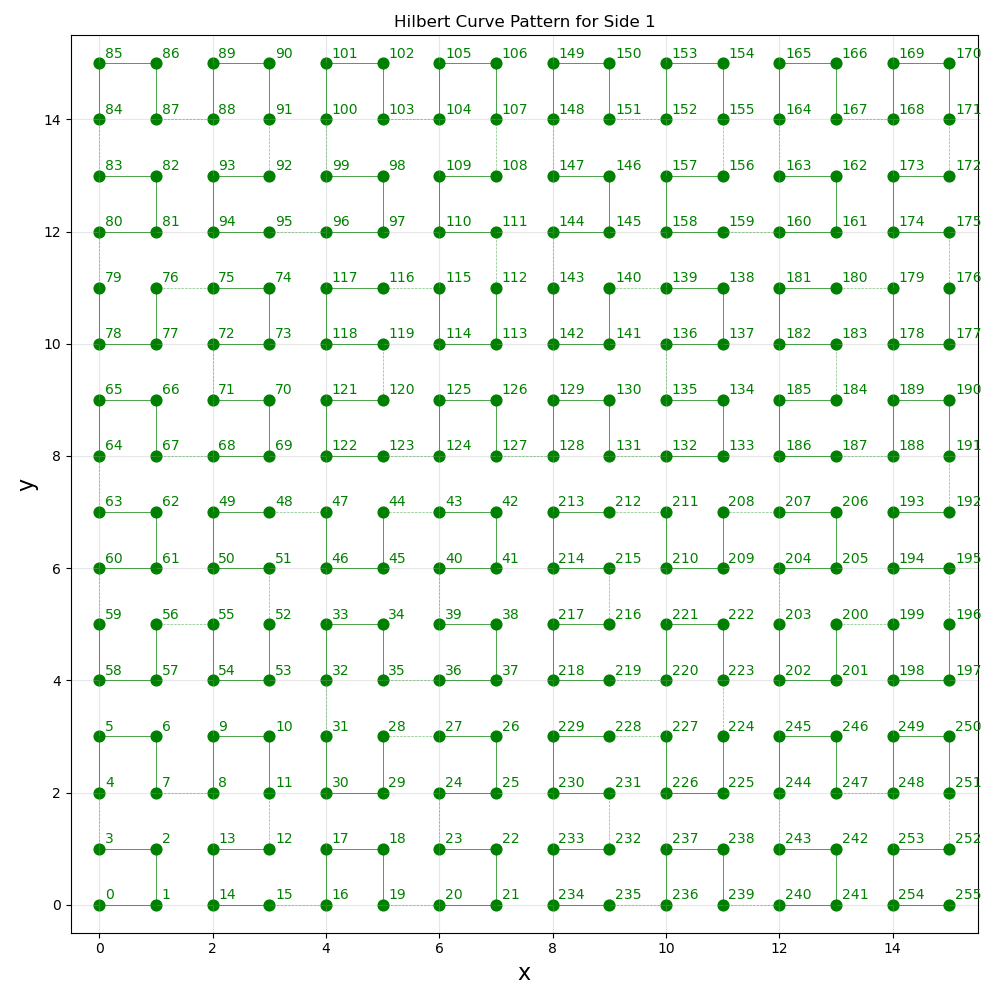
Side 1 Hilbert curve pattern
4 iterations, 2 dimensions
# Colors for tables
backs = [Back.LIGHTBLUE_EX, Back.WHITE, Back.GREEN, Back.YELLOW, Back.LIGHTMAGENTA_EX, Back.CYAN, Back.LIGHTRED_EX]
num_colors = len(backs)
Values and Number Counts
print_values()
Print a table of values for square, domino, term, and number.
def print_values():
    column_headers = ['Square', 'Domino', 'Term', 'Number']
    # array of rows
    data = []
    # num_squares is per side, but we want to tile all sides of the cube
    for square in range(0, num_squares * num_sides_dots):
        domino = get_domino(square)
        term = get_term(square)
        number = get_number(square)
        # setting different colors for different numbers (mainly because it's very easy to confuse 0 and 6 when reading the table)
        # see https://compucademy.net/python-tables-for-multiplication-and-addition/
        color = backs[number % num_colors]
        data.append([square, domino, term, f'{color}{number}{Back.RESET}'])
        # add dash to simulate 'fraction' line on domino
        if square % 2 == 1: data.append(['', '', '', '-'])
        # add spacing to make it easier to see pairs of domino numbers
        else: data.append(['........', '........', '......', '........'])
    print(tabulate(data, column_headers, tablefmt = "pretty"))

print_values()
Example output (fragment):
+----------+----------+--------+----------+ | Square | Domino | Term | Number | +----------+----------+--------+----------+ | 0 | 1 | 1 | 2 | | ........ | ........ | ...... | ........ | | 1 | 2 | 1 | 2 | | | | | - | | 2 | 2 | 1 | 3 | | ........ | ........ | ...... | ........ | | 3 | 3 | 2 | 3 | | | | | - | | 4 | 3 | 2 | 4 | | ........ | ........ | ...... | ........ | | 5 | 4 | 2 | 4 | | | | | - | | 6 | 4 | 2 | 5 | | ........ | ........ | ...... | ........ | | 7 | 5 | 3 | 5 | | | | | - | | 8 | 5 | 3 | 6 | | ........ | ........ | ...... | ........ | | 9 | 6 | 3 | 6 | | | | | - | | 10 | 6 | 3 | 0 |
print_number_counts()
Print counts of how many times each number (0 through 6) appears.
def print_number_counts():
    column_headers = ['0', '1', '2', '3', '4', '5', '6']
    # array of rows
    data = [[0, 0, 0, 0, 0, 0, 0]]
    for square in range(0, num_squares * num_sides_dots):
        number = get_number(square)
        data[0][number] += 1
    print("Number counts:")
    print(tabulate(data, column_headers))

print_number_counts()
Example output:
Number counts: 0 1 2 3 4 5 6
220 218 220 220 220 218 220
Coordinates and Squares
In local coordinates, each side's coordinates goes from [0,0] to [sqrt(num_squares) - 1, sqrt(num_squares) - 1].
In global coordinates, each side's coordinates start at a multiple of sqrt(num_squares) times the index of the side in the ordering shown in the diagram above (starting at 0). So, the first side starts at [0,0], the second at [sqrt(num_squares),sqrt(num_squares)], the third at [2 * sqrt(num_squares), 2 * sqrt(num_squares)], and so on.
Note that a single coordinate is a list of numbers (with a number of elements equal to dimensions, which for Metaphysics is always 2), e.g. [2,5]. Coordinates (plural) are lists of such lists, e.g. [[2,5], [6,3], [7,7]].
get_global_coordinates()
Given local coordinates and a side, get the corresponding global coordinates.
This function requires a list of lists input, even for a single coordinate.
def get_global_coordinates(local_coordinates, side_dots):
    global_coordinates = []
    for i in range(0, len(local_coordinates)):
        global_coordinate = []
        for j in range(0, len(local_coordinates[i])):
            global_coordinate.append(local_coordinates[i][j] + sides_dots.index(side_dots) * int(math.sqrt(num_squares)))
            if (j == len(local_coordinates[i]) - 1):
                global_coordinates.append(global_coordinate)
    return global_coordinates
set_global_coordinates()
Given local coordinates and a side, set the corresponding global coordinates.
This function requires a list of lists input, even for a single coordinate.
def set_global_coordinates(local_coordinates, side_dots):
    for i in range(0, len(local_coordinates)):
        for j in range(0, len(local_coordinates[i])):
            local_coordinates[i][j] += sides_dots.index(side_dots) * int(math.sqrt(num_squares))
set_global_coordinates_batch()
Given local coordinates and a side, set the corresponding global coordinates in a batch.
This function requires a list of a list of lists input.
Note that the order and length of the two lists (
local_coordinates_listandside_list) must match so that eachlocal_coordinatesmatches the appropriate side.
def set_global_coordinates_batch(local_coordinates_list, side_list):
    for i in range(0, len(local_coordinates_list)): set_global_coordinates(local_coordinates_list[i], side_list[i])

# Transform dots and white areas from local into global coordinates.
set_global_coordinates_batch(dots, dots_side_list)
set_global_coordinates_batch(white_areas, white_areas_side_list)
get_squares()
Given (a list of) global coordinates (e.g. a dot), find the squares (ordered along the Hilbert curve) that the list includes.
Note that either local or global coordinates can be inputted, but the output will always be global square numbers.
The input list of coordinates is in the number of the dimensions of the Hilbert curve (always 2 for Metaphysics).
The output is an (ordered) list of coordinates in 1 dimension, since the Hilbert curve itself is 1-dimensional (at least "stretched out", since the "curled up" curve has fractal Hausdorff dimension 2).
def get_squares(coordinates):
    # Calculate the side index as a kind of offset: how many times the coordinate values can be divided by sqrt(num_squares). (We can used any coordinate value to find this — coordinates[0][0] is just an arbitrary choice.) For example, if the coordinate value is 18 and sqrt(num_squares) is 16, the offset is 1 because 18 can be divided by 16 once. This ia also the side index of that coordinate: it's on the second side.
    # This index could instead be passed into the function, but it's helpful to calcuate it here so that's not necessary.
    # Note that this should always be an integer: math.trunc() and math.floor() are just safeguards.
    side_index = int((coordinates[0][0] - (coordinates[0][0] % int(math.sqrt(num_squares)))) / int(math.sqrt(num_squares)))
    local_coordinates = []
    for coordinate in coordinates:
        local_coordinate = []
        for i in range(0, len(coordinate)):
            # Mod by sqrt(num_squares) to make the coordinate local, so that distances_from_points from the hilbertcurve package can be used to calculate local square numbers.
            local_coordinate.append(coordinate[i] % int(math.sqrt(num_squares)))
        local_coordinates.append(local_coordinate)
    points = local_coordinates
    distances = hilbert_curve.distances_from_points(points)
    # Finally, calculate global square values simply by adding num_squares (per side), scaled by the side index
    global_squares = []
    for distance in distances: global_squares.append(distance + (side_index * num_squares))
    return global_squares
print_squares()
Print squares for a given list of coordinates.
The relevant group of coordinates and their names must be passed also.
def print_squares(coordinates, coordinates_group, coordinate_names):
    print('Squares for ' + coordinate_names[coordinates_group.index(coordinates)] + ':')
    print(get_squares(coordinates))

print_squares(dot_1A, dots, dot_names)
Example output:
Squares for Dot 1A: [43, 124, 41, 42, 127, 126, 214, 213, 128, 129, 212, 131]
get_other_domino_square()
Given the domino number of a square, find the other square with that domino number.
There's only one, and it's either the previous or next one.
def get_other_domino_square(square):
    previous_square = square - 1
    next_square = square + 1
    if get_domino(square) == get_domino(previous_square): return previous_square
    else: return next_square
Dominoes and Domino Counts
get_dominoes()
Given (a list of) coordinates (e.g. a dot), find the full and half dominoes that compose it.
def get_dominoes(coordinates):
    full_dominoes = []
    half_dominoes = []
    coordinates_squares = get_squares(coordinates)
    # the squares already 'used', or included in a full or half domino already added
    used_squares = []
    for square in coordinates_squares:
        other_domino_square = get_other_domino_square(square)
        # if the other domino square isn't used
        if (other_domino_square not in used_squares):
            # if it's in coordinates, add to full dominoes
            if (other_domino_square in coordinates_squares):
                domino = [get_number(square), get_number(other_domino_square)]
                # sort to avoid counting e.g. [2,5] and [5,2] separately — they should be treated as the same
                domino.sort()
                full_dominoes.append(domino)
                # add squares to used list
                # not strictly necessary to add 'square', since we're iterating over it (i.e. the for loop takes care of not considering it multiple times), but it's more intuitive to also consider it 'used'
                used_squares.extend([square, other_domino_square])
            # else, add to half dominoes
            else:
                half_domino = get_number(square)
                half_dominoes.append(half_domino)
                used_squares.append(square)
    return full_dominoes, half_dominoes
get_dominoes_counts()
Given (lists of) full and half dominoes (e.g. for a single dot), count how many there are of each type.
Order doesn't matter for full dominoes, e.g. [2,5] and [5,2] are considered the same. This will be used in table data, so notice that there are row headers included (which aren't themselves counts, of course).
The table data for half dominoes has only one row, so there's no need for a row header there.
def get_dominoes_counts(full_dominoes, half_dominoes):
    # the first values are row headers
    full_dominoes_counts = [[0], [1], [2], [3], [4], [5], [6]]
    # no need for row headers — there's only one row
    half_dominoes_counts = [[]]
    for i in range(0, 7):
        for j in range (0, i + 1):
            # They're already sorted in get_dominoes(), so no need to count both [i,j] and [j,i].
            # If it seems odd that it's [j,i] below, that's only because j is never greater than i given this iteration strategy, so it should come first because sort(), used in get_dominoes(), puts smaller numbers first (i.e. ascending order).
            full_dominoes_count = full_dominoes.count([j,i])
            # Using append() here takes care of the ordering, so no need to use the j index.
            full_dominoes_counts[i].append(full_dominoes_count)
        half_dominoes_count = half_dominoes.count(i)
        half_dominoes_counts[0].append(half_dominoes_count)
    return full_dominoes_counts, half_dominoes_counts
get_sum_dominoes_counts()
Given (a list of a list of) coordinates (e.g. a list of dots), find the sum of counts for full and half dominoes.
def get_sum_dominoes_counts(coordinates):
    # initilialize with zero values so they can later be overwritten (to avoid 'index out of range' error)
    sum_full_dominoes_counts = [
        [0, 0],
        [1, 0, 0],
        [2, 0, 0, 0],
        [3, 0, 0, 0, 0],
        [4, 0, 0, 0, 0, 0],
        [5, 0, 0, 0, 0, 0, 0],
        [6, 0, 0, 0, 0, 0, 0, 0]]
    sum_half_dominoes_counts = [[0, 0, 0, 0, 0, 0, 0]]
    for i in range(0, len(coordinates)):
        full_dominoes, half_dominoes = get_dominoes(coordinates[i])
        full_dominoes_counts, half_dominoes_counts = get_dominoes_counts(full_dominoes, half_dominoes)
        # add up full domino counts
        for j in range(0, len(full_dominoes_counts)):
            # start at 1 since the first items are just row headers
            for k in range(1, len(full_dominoes_counts[j])):
                # adjust by frequency
                sum_full_dominoes_counts[j][k] += (full_dominoes_counts[j][k])
        # add up half domino counts
        for l in range(0, len(half_dominoes_counts[0])):
            # adjust by frequency
            sum_half_dominoes_counts[0][l] += (half_dominoes_counts[0][l])
    return sum_full_dominoes_counts, sum_half_dominoes_counts
print_dominoes_counts()
Given (a list of a list of) coordinates (e.g. a list of dots), print tables of full and half domino counts.
The "names" input is a list of names for each list of coordinates.
def print_dominoes_counts(coordinates, names):
    full_dominoes_headers = ['#', 0, 1, 2, 3, 4, 5, 6]
    half_dominoes_headers = [0, 1, 2, 3, 4, 5, 6]
    for i in range(0, len(coordinates)):
        full_dominoes, half_dominoes = get_dominoes(coordinates[i])
        full_dominoes_counts, half_dominoes_counts = get_dominoes_counts(full_dominoes, half_dominoes)
        print('Full Dominoes for ' + names[i] + ':')
        print(tabulate(full_dominoes_counts, full_dominoes_headers))
        print('Half Dominoes for ' + names[i] + ':')
        print(tabulate(half_dominoes_counts, half_dominoes_headers))
    sum_full_dominoes_counts, sum_half_dominoes_counts = get_sum_dominoes_counts(coordinates)
    print('Full Dominoes for All:')
    print(tabulate(sum_full_dominoes_counts, full_dominoes_headers))
    print('Half Dominoes for All:')
    print(tabulate(sum_half_dominoes_counts, half_dominoes_headers))

print_dominoes_counts(dots, dot_names)
print_dominoes_counts(white_areas, white_area_names)
Example output (fragment):
Full Dominoes for Dot 1A:
0 1 2 3 4 5 6
0 0 1 0 0 2 1 0 1 3 0 0 0 0 4 0 0 0 1 0 5 0 0 0 0 0 0 6 0 0 0 0 0 0 0 Half Dominoes for Dot 1A: 0 1 2 3 4 5 6
1 0 2 1 1 1 0 Full Dominoes for Dot 2A:
0 1 2 3 4 5 6
0 0 1 0 0 2 0 1 0 3 1 0 0 0 4 0 0 0 0 0 5 0 0 0 0 0 0 6 1 0 1 0 0 0 0 Half Dominoes for Dot 2A: 0 1 2 3 4 5 6
... Full Dominoes for All:
0 1 2 3 4 5 6
0 1 1 4 3 2 3 3 1 3 3 4 3 3 4 3 3 5 3 1 5 2 1 5 5 3 2 6 4 3 3 1 3 3 3 Half Dominoes for All: 0 1 2 3 4 5 6
13 14 11 12 13 17 10 Full Dominoes for White Area for Side 1:
0 1 2 3 4 5 6
0 3 1 6 3 2 4 5 2 3 4 5 5 3 4 3 5 3 6 3 5 4 4 3 5 6 3 6 6 5 4 4 5 6 3 Half Dominoes for White Area for Side 1: 0 1 2 3 4 5 6
1 0 3 1 2 1 0 Full Dominoes for White Area for Side 2:
0 1 2 3 4 5 6
0 2 1 4 2 2 5 4 2 3 4 5 5 2 4 6 5 5 3 2 5 4 7 6 5 4 2 6 4 4 4 4 4 5 2 Half Dominoes for White Area for Side 2: 0 1 2 3 4 5 6
0 1 1 3 1 3 1 ... Full Dominoes for All:
0 1 2 3 4 5 6
0 10 1 25 10 2 27 25 14 3 27 25 25 10 4 24 25 19 25 12 5 23 25 22 20 24 11 6 25 23 25 27 27 26 10 Half Dominoes for All: 0 1 2 3 4 5 6
15 12 14 14 17 16 14
get_min_num_sets()
Given counts of full and half dominoes, find the minimum number of domino sets required.
A standard domino set (with column and row headers) is:
#   #    0    1    2    3    4    5    6
# ---  ---  ---  ---  ---  ---  ---  ---
#   0    1
#   1    1    1
#   2    1    1    1
#   3    1    1    1    1
#   4    1    1    1    1    1
#   5    1    1    1    1    1    1
#   6    1    1    1    1    1    1    1
That is, it has one domino of each type. As a result, there are 8 half dominoes of each number (0 through 6).
def get_min_num_sets(full_dominoes_counts, half_dominoes_counts):
    # The minimum number of sets must be at least as great as the highest full dominoes count. (That's because there's no other way to get a particular full domino than through a new set, since each set has only one of a given type.)
    max_full_dominoes_count = 0
    for i in range(0, len(full_dominoes_counts)):
        # start at 1 since the first items are just row headers
        for j in range(1, len(full_dominoes_counts[i])):
            if full_dominoes_counts[i][j] > max_full_dominoes_count: max_full_dominoes_count = full_dominoes_counts[i][j]
    min_num_sets = max_full_dominoes_count
    # how many half dominoes are left over for use
    # initilialize with zero values so they can later be overwritten (to avoid 'index out of range' error)
    leftover_half_dominoes_counts = [[0, 0, 0, 0, 0, 0, 0]]
    # Loop through again and set each leftover full dominoes count to be the difference between the (provisional) minimum number of sets and the value of the corresponding full dominoes count.
    for k in range(0, len(full_dominoes_counts)):
        # start at 1 since the first items are just row headers
        for l in range(1, len(full_dominoes_counts[k])):
            # k and l - 1 (minus 1 because there aren't row headers for the leftover half dominoes counts list) are the domino numbers, so add to those leftover half dominoes counts
            leftover_half_dominoes_counts[0][k] += max_full_dominoes_count - full_dominoes_counts[k][l]
            leftover_half_dominoes_counts[0][l - 1] += max_full_dominoes_count - full_dominoes_counts[k][l]
    # Check if there are enough leftover half dominoes.
    for m in range(0, len(half_dominoes_counts[0])):
        while half_dominoes_counts[0][m] > leftover_half_dominoes_counts[0][m]:
            # If there aren't enough leftover half dominoes with a particular number, we don't have enough sets. So, increment the minimum number of sets by 1 and the leftover half dominoes counts by 8 (since each set has 8 half dominoes of a particular number)
            min_num_sets += 1
            for n in range(0, len(leftover_half_dominoes_counts[0])): leftover_half_dominoes_counts[0][n] += 8
    # Once we have enough leftover half dominoes for each number, we have the minimum number of sets.
    return min_num_sets
print_min_num_sets()
Given (a list of a list of) coordinates (e.g. a list of dots), print the minimum number of sets to cover them.
def print_min_num_sets(coordinates):
    sum_full_dominoes_counts, sum_half_dominoes_counts = get_sum_dominoes_counts(coordinates)
    min_num_sets = get_min_num_sets(sum_full_dominoes_counts, sum_half_dominoes_counts)
    print('Minimum Number of Domino Sets to Cover All:')
    print(min_num_sets)

print_min_num_sets(dots)
print_min_num_sets(white_areas)
Example output:
Minimum Number of Domino Sets to Cover All: 5 Minimum Number of Domino Sets to Cover All: 27
Whew! After all that, we now know that it should take 5 black and 27 white domino sets to make the die of dominoes (at the scale of 16 by 16 squares, using Hilbert curves of 4 iterations). And that's exactly how many sets it took.